The US GDP Growth and Sustainability Debt

1. Introduction

Public debt levels rose during the 2007/2008 financial crisis and its aftermath. The decline in economic activity was reflected in the decline in economic growth rates (see Figure 1). Against this background, researchers and policymakers wanted to know more about the potential impact of higher public debt-to-GDP ratios on growth (eg Reinhart et al. 2012; Panizza and Presbitero 2013). In a key contribution, Reinhart and Rogoff (2010) present a long historical data series to analyse ratios of public debt to GDP and economic growth. Their discovery that public debt-to-GDP ratios of more than 90% are associated with significantly lower rates of economic growth has generated considerable controversy. While many prominent US and European policymakers have directly referred to Reinhart and Rogoff (2010) in advocating immediate fiscal consolidation measures to control public debt (e.g. Konzelmann 2014), several groups of researchers have used the data provided by Reinhart and Rogoff (2010) as well as newly established datasets to perform extensive econometric tests on the impact of public debt levels on economic growth (e.g. Kumar and Woo 2010; Herndon et al. 2014; Pescatori et al. 2014; Eberhardt and Presbitero 2015; Amann and Middleditch). 2020). However, the literature—including the most cited papers—partially reports contradictory results. Several papers argue that there is evidence of a negative causal effect of higher public debt-to-GDP ratios on economic growth (e.g., Afonso & Gales 2013; Wu & Kumar 2015; Chodek et al. 2017), and (close to) the 90% threshold in The ratio of public debt to GDP beyond which growth slows significantly (e.g. Caner et al. 2010; Checherita-Westphal and Rother 2012; Baum et al. 2013). While other studies acknowledge the stereotyped fact of a negative association between initial public debt levels and subsequent growth, they argue that the evidence for a causal effect extending from higher public debt to GDP to economic growth is weak at best (eg Panizza and Presbitero 2014; Ash et al. al. 2020). Furthermore, several authors point to systematic differences in the (nonlinear) effect of public debt on growth across countries, implying a lack of evidence for general thresholds in the public debt-to-GDP ratio beyond which growth falters (eg Pescatori et al. 2014; Eberhardt & Presbitero 2015; Egert 2015a; Yang & Su 2018; Eberhardt 2019; Ash et al. 2020; Bentour 2021).

The occupant of economists for the last decades has always been the impact of the rising continuation of the US debt and whether any plan from the government to alter this rising by implementing a new system, or leave the situation as it is.

Different conflicted thoughts and opinions, some of them see the government should reconsider the unfunded obligation, unproductive spending, the hikes in the interest rate and inflation raising and the fluctuations of the situation. On the other hand, others see the government should reconsider the low-interest rate or the stability and strength of the government and the dollar. We need to examine both opinions and analyse them deeply and structurally. This paper was written -including all projections- in November 2021.

The USA is different from other countries, its government doesn't necessarily need to pay the entire debt, while the government service the debts and keeps the creditors satisfied. The government should be assured of having enough cash flow to maintain the debts by making the payments on time annually, while the interest rate fluctuated and the stability of the GDP growth with considering upcoming events such as COVID-19 and recession.

The US debt hit the highest number in history and the annual service of this debt approached enormous figures. This is due to the last unproductive spending by President Trump the historical three and a half trillion dollars (COVID-19 related) and the stimulus package by President Biden for two trillion dollars is offset by uncertain income such as tax cuts which was imposed by President Trump.

the perspective projection of the US debt to be increased reach 2030 over ten trillion dollars ($10.6), with more than eight hundred billion dollars ($829) on the annual payment for maintaining the debt and satisfying the creditors, which means increasing the annual payment from the US budget by double of what is paid today regarding the interest rate payment. This payment does not reduce the debt amount, or even reduction on the budgetary spending, on the other hand, expectancy increases on average life, which means to increase in the spending services such as pensions, healthcare and social security, with the accelerated benefit of unemployment since the pandemic.. etc. the projection of Gini coefficient to reach 0.5, which means the disparity of income and that prevent the US government abilities to maximize the collection efficient tax (Efficient Tax is when the government receives a higher level of return from an individual taxpayer than it pays out to that taxpayer in benefits). Furthermore, the investments into productivity and growth to control and reduce unemployment and decreased social security spending while increasing the institutions' growth, while all these as a very small percentage contribution to the federal government budget, represent a little amount to justify the debt. Meanwhile, investing in the technology and science sector will not help to justify the debt as represents just 1% of the federal budget, even investment in sectors such as training, employment, social services and education also represent 4% of the federal budget.

Such a structure of the budget will hinder the growth of the economy in the long run, this can be clear by seeing the growth model of neoclassical (Neoclassical Growth model is a product of the function Y = AF (K, L)). The growth model of the neoclassical relies on the concept that the growth of the economy is driven by (L) labour, (A) technology and (K) capital.

While the investment in technology innovation, training and education represents 5% of the federal budget, unemployment increased massively meanwhile the flow of FDI in general reduced to 49% globally, therefore the innovation sector suffered from a lack of funding, which also damaged the openness to of the economics when implementing protectionist policies, also resulted in hinder the growth. The expectation of a fall in personal income that contributes to the GDP per capita being below ($18) thousand dollars, moreover harming prospect of the growth and also the output can dramatically be affected unless taking a further step by restructuring the budget

In general, the imbalance between outflows and inflows could lead the government to a scenario to choose between reducing the outflows such as refusing to pay income security (social security) or Medicaid (medical benefits), while millions of families to be suffered, they relied on the medical benefits to survive, or reducing the basic functions funding such as national parks and defence.

If they chose instead to default or delay payments of the debt interest, the fallout on the economy will be massive. With the fall of the credit rates, a crash in the stock market inevitably, hiking of the interest rate. On April 26, 1979, The US treasury inadvertently missed payments and thus defaulted because the back office of the Treasury was on the fritz. The mishap in part was due to the raising delay of the debt limit, and also to a technic mistake of the treasury equipment. The investors received their payment shortly after, but even so, the volatility on the T-bill yields at that time jumped to 60 base points, which cost the taxpayer multi tens of billions of dollars.

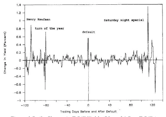
Finally, the standard debt measurements which are less prevailing don't contain unfounded obligations, such as the money promised by the federal government of the US, but will unlikely be able to pay off (such as medical benefits and retirement). Less than the current stock available Medicare and social security funds, which predicted returns of 80 to 200 trillion, while Fannie Mae and some other organisations of the government owe around 3 to 8 trillion in the obligation that is not funded, total yielding 165 trillion.

2. Literature Review

The literature on the relationship between public debt and economic growth has grown significantly in the aftermath of the 2007/08 financial crisis (e.g., Reinhart et al. 2012; Panizza & Presbitero 2013; Amann & Middleditch 2020). A comprehensive survey of the literature would be beyond the scope of this paper. The discussion in this section will focus on presenting those parts of the theoretical literature that have broadly guided econometric testing, and on presenting and contextualizing the most important elements of the relevant empirical literature.

The “traditional view” of government debt emphasizes public debt's positive aggregate demand effects in the short run and crowding out effects that discourage economic activity in the long run (Elmendorf & Mankiw 1999). From this point of view, an increase in the budget deficit leads to an increase in disposable household income, especially when there is a recession in the economy. The corresponding increase in income and wealth boosts aggregate demand for goods and services. While the "traditional view" regards economics as Keynesian in the short run, the outlook is still "classical" in the long run: public savings fall due to the increase in the fiscal deficit, but private savings do not rise enough to compensate for the decline in public savings; Therefore, national savings decline; Total investment is reduced, which leads to lower capital and lower output growth.

The long-term negative effect of public debt on growth could be due to crowding-out mechanisms: if rising fiscal deficits lead to higher interest rates, this could crowd out private investment. Moreover, net exports may decrease due to the appreciation of the exchange rate. If more government debt is associated with higher inflation, this could also act as a drag on growth (e.g., Ash et al. 2020). Cochrane (2011) argues that the negative impact of a high level of public debt on growth can be very significant if the high debt enhances uncertainty and expectations of higher inflation and financial repression. However, in the "unorthodox view" of government debt, an initial increase in fiscal deficits that initially leads to a higher level of public debt - particularly when the output gap is large - not only temporarily increases aggregate demand, but increases Long - the rate of running growth through deceleration (eg Delong & Summers 2012; Fazzari et al. 2020). Some endogenous growth models also yield results consistent with a positive effect of public debt on growth in the transition to the new steady state, depending on what debt is actually financed (Aizenman et al. 2007).

The idea that has strongly guided the test in the econometric literature is that there can be thresholds in the public debt-to-GDP ratio beyond which growth declines significantly. However, finding fully defined theoretical models that give predictions for such thresholds is not easy at all. Theoretically, nonlinearity could arise due to the burden of public debt (eg Krugman 1988). Ghosh et al. (2013) present a formal model where nonlinear aspects emerge when a tipping point is reached beyond which public debt becomes unsustainable; However, their theoretical argument is not an integral part of the growth framework. Checherita-Westphal et al. (2014) constructed a theoretical model in which public debt can only be issued for spending on public investment; The ratio of public to private capital determines the optimal level of public debt to GDP. In their model, the optimal level of debt-to-GDP that maximizes GDP growth depends on the production elasticity of the capital stock. In building on Checherita-Westphal et al. (2014), Greiner (2013) argues that this theoretical outcome is driven by the assumption that fiscal deficits equal public investment. Relaxing this assumption—that is, allowing governments to take on debt for things other than a public investment—produces a monotonously negative relationship between public debt to GDP and the steady-state growth rate. Teles & Mussolini (2014) present a model in which generational and endogenous growth overlap, in which higher levels of public debt to GDP extract some of the savings of the younger population (which is needed to pay interest), resulting in exhaustion. The effect reduces the impact of productive government spending on economic growth. Proaño et al. (2014) constructed a dynamic growth model in which public debt levels have a non-linear impact on economic activity through inflations from the financial sector, where a rise in public debt to GDP weakens growth only in times of financial stress. Alesina et al. (1992) argue that higher levels of public indebtedness can be linked to perceived default risk by investors, giving rise to nonlinear factors.

Another potential channel through which high levels of public debt could ultimately have a negative impact on growth is its effect on countercyclical fiscal policy: if high debt levels constrain the government's ability to use expansionary fiscal policy in recessions, it could To increase the volatility of production and thus reduce growth (e.g. Ramey and Ramey 1995). In a world of multiple equilibria, a fully solvent government with a high level of public debt may decide to implement restrictive fiscal policies to reduce the possibility that a sudden change in investor sentiment will push the country into a state of poor equilibrium. However, it can be argued that the government's ability and willingness to use expansionary fiscal policy in recessions depends more on monetary arrangements (in particular: on coordination with the central bank) and public debt structures than on the actual level of public debt-to-GDP ratio aggregate (e.g. de Grauwe 2012).

3. The Effect of Higher Public Debt Levels on Growth

In influential research, Kumar & Woo (2010) start from the emerging fact that there is a negative relationship between primary government debt and real GDP per capita growth—suggesting that a 10-percentage-point delayed increase in the public debt-to-GDP ratio, on average, they are associated with lower GDP growth rates by 0.25 percentage points (Kumar and Wu 2010, 8-9). However, the authors rightly note that this relationship ignores potential homogeneity issues between public debt and growth: the ratio of public debt to GDP and economic growth outcomes can be jointly determined by third factors. Moreover, the explanations for causation are by no means clear, since stagnation in economic activity may be largely responsible for increases in public debt to GDP—the so-called reverse causation problem. However, Kumar & Wu (2010) argue that they address reverse causality and homogeneity issues by using delayed levels of public debt and a GMM estimation approach with appropriate instrumental variables. In doing so, they report findings indicating that increases in public debt to GDP are indeed associated with a slowdown in annual real GDP growth. Other empirical papers support this finding of a negative linear effect of the public debt-to-GDP ratio on real GDP growth (Cecchetti et al. 2011; Afonso & Jalles 2013; Afonso & Alves 2015; Woo & Kumar 2015; Chudik et al. 2017).

However, Panizza & Prespitero (2014) call interpretations of the negative causal effect of the public debt-to-GDP ratio on growth into question. They argue that literature that has attempted to address homogeneity using lagging values of public debt to GDP (Cecchetti et al. 2011), internal tools via GMM estimation (Kumar & Woo 2010), or by measuring public debt with average debt-to-GDP ratios have failed The overall results in other countries (Checherita-Westphal & Rother 2012) failed to produce findings that convincingly address heterogeneity. Therefore, Panizza & Presbitero (2014) propose a new strategy to address the homogenization problem: using an external tool for the public debt-to-GDP ratio based on the fact that when there is a public debt denominated in foreign currency, changes in a country's exchange rate directly affect the ratio. public debt to gross domestic product. They show that when they use the new median variable, the association between debt and growth disappears such that there is no evidence of a negative causal effect of public debt on economic growth.

Ash et al. (2020) address issues of coherence and reverse causation using indicators and lagging GDP growth in relation to public debt. provides a comprehensive assessment of the impact of public debt on growth using various data sets from influential papers in the literature, including Reinhart & Rogoff (2010), Cecchetti et al. (2011), Checherita-Westphal & Rother (2012) and Woo & Kumar (2015). They report the findings that the relationship between the ratio of public debt to GDP and growth is close to zero since the 1970s, and there is no evidence of a causal effect of public debt on growth. Ash et al. (2020) argue that previous findings in the literature suggesting a negative impact of public debt on growth are sensitive to small samples, outliers, and exotic econometric choices.

Eberhardt & Prespitero (2015) appreciate empirical characteristics that allow for heterogeneity in the long-term relationship between public debt and economic growth across countries. They provide evidence of systemic differences in the effect of public debt on growth across countries. Therefore, the same policy response may not be appropriate in all countries. Other studies that allow the impact of public debt on growth to vary across countries also underscore this point (Bell et al. 2015; Sosvilla-Rivero & Gomez-Puig 2019; Bentour 2021).

4. Methodology

The Congressional Budget Office (CBO) regularly publishes reports that provide projections of the federal budget deficit, debt, revenue and spending — and the economic trajectory that underlies it — for the current year and the next 10 years if existing laws governing taxes and spending, in general, remain unchanged. For this report, the latest in the series, projections are based on laws in force as of January 12, 2021. The CBO's economic assessment is identical to the forecast published by the agency on February 1, 2021.

Our long-run estimates include dynamic feedback from choices about budget policies to GDP and interest rates. These are chosen to be very conservative and come closer to standard estimates so do not reflect the fact that higher debt, for example, enables more effective monetary policy and thus smaller output gaps and a higher level of long-run output. In CBO projections, the annual deficit averages $1.2 trillion annually from 2022 to 2031 and exceeds the 50-year average of 3.3% of GDP in each of those years. It declines to 4.0% of GDP or less from 2023 to 2027 before rising again, to 5.7% of GDP in 2031. By the end of the period, both the primary deficit (which excludes net expenditure for interest rises) and interest expenses. From an economic view. As expanded vaccination reduces the spread of COVID-19 (the disease caused by the coronavirus) and the extent of social distancing decreases, real (inflation-adjusted) GDP is expected to grow by 3.7% in 2021, returning to the pre-pandemic level before the middle of the year. With a growth rate of 2.6% over the period 2021-2025, real GDP exceeds its potential (sustained maximum) level in early 2025. The unemployment rate gradually decreases until 2026, and the number of working people returns to the prepandemic level in 2024.

Average real GDP growth of 1.6% over the period 2026-2031. This average output growth rate is lower than its long-term historical average, mainly because the labour force is expected to grow more slowly than it did in the past. During the forecast period, the interest rate on 10-year Treasury notes is expected to gradually increase to 3.4% in 2031.

Changes since previous CBO projections. As for its estimates from September 2020, the CBO's estimate of the deficit for 2021 is now $448 billion (or 25%) greater, and its cumulative deficit forecast between 2021 and 2030 (at $12.6 trillion) is now $345 billion (or 3%). ) smaller. In 2021, the costs of recently enacted legislation are partially offset by the effects of a stronger economy. In subsequent years, the biggest changes stem from economic forecast revisions. The CBO now expects stronger economic activity, higher inflation and higher interest rates, which should boost revenues and expenditures - the former more than the latter.

5. Justifying the Debt Raising

These data are alarming and rendering for action instantly, we should always consider the values of forecasted brings bundles of uncertainties, while CBO predicted the values of the Debt to GDP more the 77 points. Moreover, economic growth is stable in the US. Nevertheless, increasing the interest rate is a suicide move, which could solve the inflation problem for some time but will lead to a big recession in future.

The testimony is almost all consistent with the change of the structural propensities to invest and save as the predominant cause of the real rates declines. (AAs Summers 2014), the factors which affect to raise in inequality increase, in private savings include retirement with longer periods and rising uncertainty.

Factors operating to reduce private investment include slowing labour force growth, greater efficiency in the use of capital, for example through companies like Uber and Airbnb, and the impact of information technology in reducing the need for large capital investments, for example, law firms need much less office space per lawyer and dramatic reductions in the relative price of capital goods. Increases in corporate market power and increased pressure on corporations to pay out cash to shareholders may also contribute to reduced investment. This along with inflation drastically affects the amount that can be borrowed. Simply put, real interest rates compare the real interest being paid on debt to GDP, and therefore to compare this to standard nominal interest rate measurements as a ratio of GDP, we use a simple formula:

The use of real interest rates shows us how inflation, which is projected to fluctuate around 2% until 2030, is gradually also wiping out US debt in large amounts bringing real interest payments to almost 0% as a ratio of GDP. This makes large amounts of borrowing and debt-to-GDP ratios sustainable and one can see that throughout the 2000s despite interest rates being at 4.3% for US treasuries and inflation rates being at 2.46%, the FED was easily able to pay off its debt. Nevertheless, the low-interest rates don't mean borrowing a luxury, they make it mandatory. For example, the GDP contracted more than 30% in Q2 of 2020 (second quarter of 2020) due to the pandemic courtesy of both demand shocks and interruptions in supply chains, leading to widespread job losses and sparse spending. Already low-interest rates were meant to revive the economy, but monetary policy in itself simply wasn’t enough. Therefore increased government spending in grants and other investments (Approximately $150 billion more than FY19) through undertaking increased debt become a necessity to help the economy recover. A more complicated model proposed by Furman and Summers based on the measure of debt satisficing and can be compared to GDP growth on an infinite scale shows that a ‘0.5 percentage point increase in tax revenue as a share of GDP or reduction in spending as a share of GDP would be sufficient to pay 21 off the entire debt.

Alongside individual parameters, the situation in the US can also be analysed by comparing it to other nations, specifically the G7 or even G20 nations since they provide the most accurate socio-economic comparison to the US as in Figures 2 and 3. Although the US has the fastest expected GDP growth rate, it also has the second-largest debt-to-GDP ratio behind Japan and tax revenue as a percentage of GDP falls below even OECD levels at 31% as compared to the average 37%. Nevertheless, payments of the real interest approximation almost 0% ratio-wise with the GDP, thus making the US financial status more strongly than most of the other nation of G7 nations in terms of capacity to satisfice debt.

Finally, the US dollar is also the reserve currency of the world, and US treasuries are widely considered one of the safest investments. Therefore because it is the backbone of a large part of international trade and transactions, the US dollar holds a strong and constant level of demand, ensuring its value does not crash. The credit rating and reputation of the US government along with the demand for the dollar ensure that government-issued bonds are also always purchased by both international and national stakeholders, ensuring that debt can continuously be sanctioned by the US government at low-interest rates.

6. Fiscal Policy Guidepost (Interest Below 2% of GDP)

However, the space for fiscal expansion is not unlimited and policymakers need evidence for assessing fiscal sustainability, particularly when the fiscal policy objective is consistent with many different levels of debt and there is no single defined fiscal path. When the growth rate is greater than the interest rate, there is much more scope to run a primary deficit and any given primary deficit will not lead to an unlimited explosion of debt but instead will bring the debt closer to a finite value. However, the finite value that debt implies can be very large - and large enough that the upward pressure it exerts on interest rates is unlikely to keep growth rates above interest rates in which case the resulting dynamic is an explosion in debt and interest payments.

We suggest the following approach: Policymakers need not worry about the fiscal outlook as long as the ratio of debt service to GDP, measured in real terms, is expected to remain comfortably within historical experience over the next decade and not spiral upward over that period. This can be triggered roughly as it restricts real interest payments to comfortably below 2% of GDP measured ideally in the economic sense of net interest less remittances from the Federal Reserve and interest on federal financial assets (see Appendix I). To the degree that there is room to increase revenue, a country can have more room to supply and to the extent that there are significant headwinds from bond markets crowding out investment, it has less room to supply. If interest payments become expected to exceed our approximate ceiling, policies directed at lowering the debt-to-GDP ratio would be appropriate. It is an advantage, not a fault, that our approach does not provide a prescription for the appropriate level of debt-to-GDP itself.

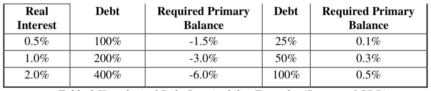
Debt levels and primary budget balances associated with various real interest rate targets depend on the real interest rate and growth rate. When real interest rates are low, there is much more room to raise debt levels without triggering excessively high real interest as a share of GDP. The higher the growth rate, the greater the primary deficit that can correspond to this interest and debt path. The different primary deficits required in the steady state, the resulting debt levels for the alternative real debt service objectives, the assumed interest rates, and growth rates are shown in Table 1.

Debt dynamics can be analysed using the previously discussed identity:

In the steady state with a stable debt-to-DGP ratio, this becomes

If real interest rates remain below 1.33% - currently much higher than expected - a debt level of 150% of GDP will be comfortably sustainable by our standards. If, unreasonably, real interest rates were still 0.5 per cent as the debt-to-GDP ratio rose to 400 per cent, that would suggest that ultra-low interest rates were such a powerful force that this degree of debt would be justified As shown in Table 1. Conversely, if real interest rates rise to 2%, the debt-to-GDP ratio should be lower because all the problems associated with lowinterest rates will be diminished, so the debt-to-GDP ratio of 100% will be more reasonable.

Illustrative Scenario 1 Illustrative Scenario 2

Typeset table reconstructed from version-of-record PDF page 13. Select the image to open the full-resolution facsimile.

Accessible table text

Table 1 Hypothetical Debt Sustainability Examples (Percent of GDP)

Real Interest	Debt	Required Primary Balance	Debt	Required Primary Balance
0.5%	100%	-1.5%	25%	0.1%
1.0%	200%	-3.0%	50%	0.3%
2.0%	400%	-6.0%	100%	0.5%

7. A New Fiscal Policy Guidelines for The US

Operating a financial plan that advances the broad goals we have set for fiscal policy while adhering to the sustainability guidelines we propose depends on projections of the financial situation. In the United States, total US debt service obligations are currently modest and debt relative to future GDP and the ability to generate taxes from that GDP. Even the most traditional and misleading measure of the debt-to-GDP ratio is stable over the next decade and assuming compliance with existing law, which requires tax cuts and Social Security reform to expire, will be essentially stable over the next decade. Three decades too, although it could reasonably be anywhere from among the lowest in postwar history to about 190% of GDP. The additional investments of around 1% of GDP that initially lifted debt above this path could pay for themselves, and to the extent they do not, interest as a share of GDP will remain below historical levels.

Given current projections, a set of three broad guidelines would help move fiscal policy toward a better position to achieve our goals while providing a constraining principle for determining policy. Our starting point is the current law, which includes the expiry of the 2017 tax cuts and Social Security reform. Debt is largely stable on the assumption that policymakers are law-abiding and concerns about debt stability are based largely on concern that they will pass laws in the future that lead to a higher debt path.

We then propose three general guidelines for the conduct of fiscal policy in practice that can be operationalized as more specific rules:

1. Temporary emergencies should not be paid for, with a broad definition of what

constitutes a temporary emergency and what can be done in the situation. As discussed above, more fiscal support is needed today - and likely will be needed going into future recessions. In many cases, this fiscal support may effectively pay for itself resulting in a lower debt-to-GDP ratio and perhaps a lower real net interest as a share of GDP as well. A dynamic valuation using demand-side models would be appropriate to assess the fiscal impact of short-term emergency spending. Given the likely lingering effects of current and future downturns, the potential for reductions in potential GDP, and the amount of fiscal room, it would be logical for policymakers to err on the side of a broad definition of unpaid emergency spending that lasts for several years and includes items that are not spent immediately, Like spending on infrastructure.

1. Permanent programs should be paid for, with wide exceptions for programs that

reasonably pay for themselves in net present value, such as investments in children. The principle of paying for permanent changes makes broad sense and is consistent with a sustainable real debt service path given current expectations. Further, a constraining principle is needed for budget preparation and as a way of evaluating whether any particular program or proposal makes sense. In principle, firmware should be evaluated using dynamic registration. In practice, this dynamic valuation can be difficult to do in real-time and misses the fact that much of the return on investments happens outside the budget window. As a result, we propose a crude way to account for this by excluding a select group of programs and investments from pay-as-you-go restrictions when strong evidence from academic research indicates that they would reasonably pay for them in present value terms. This includes welldesigned investments in areas such as children, education and research. Ideally, the infrastructure would be paid for through Pigouvian revenue measures that optimize infrastructure utilization, but it also could get an exception to the pay-as-you-go principle.

1. Improving the composition of the government to make it more supportive of demand

and more efficient. This includes many of the steps discussed earlier in this paper: improving automatic stabilizers to better respond to recessions and increased demand through balanced expanded budget multipliers, gradual fiscal transfers and expanded social insurance. Creating what government does is important and to make room for additional investment many changes need to be made in their interest, such as reforming healthcare delivery systems in a way that will save costs and possibly improve or not deteriorate quality. Better results and enforcement of the tax system to collect what is owed under the current law (Sarin & Summers 2019).

Figures 4a, 4b and 4c show the resulting debt, nominal interest, and real interest trajectories under a program consistent with these guidelines. We believe that policymakers should focus only on the next decade due to the growing uncertainty about budget deficits after that period but we still provide thirty years of estimates to show the current best guess of the long-term impact of this program, which is a topic of interest for some policy analysts. Specifically, by way of illustration, these estimates assume an additional $2.5 trillion in fiscal support over the coming years there and an investment program that starts at a net cost of 1% of GDP but eventually begins to cause deficit reduction over a longer period. Overall, this could mean about $5 trillion in deficit-financed investment over the next decade-plus additional investment paid through added revenue or other spending cuts. The result is that debt will stabilize at less than 150% of GDP, the highest level the US has ever seen, but nominal interest payments will still be just 3.8% of GDP, and real interest payments will be just 1.0% of GDP. Total (around the 77th percentile of historical experience).

8. Future Speculation

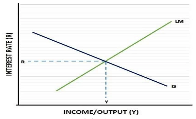
Future effects of this continual borrowing can result in drastically varying conditions to those which the government borrows now. This can be represented through the IS-LM model in Figure 5. Increased borrowing and money flow, along with average hourly earnings climbing steadily due to post-pandemic labour market recoveries means inflation is bound to accelerate. While this may be beneficial in terms of real interest rate payments it creates a whole host of problems including absolute poverty and the depreciating value of the US dollar. In order to counteract these problems, the FED has planned to double the pace of taper to $30 billion a month. Along with this three interest rate hikes are planned by the end of 2022 to control the money supply and bring equilibrium to a prospective LM curve for the US economy. The direct effect of this can be modelled using an IS curve, which shows that GDP and output reduce as interest rates grow and firms reduce investment and consumers prioritize saving. The Phillips curve can further be used to show the inverse relationship between unemployment and inflation, and as the government aims to control inflation rates, unemployment increases, resulting in an increased need for income security. All of these direct effects show a worrying prospect for the US budget.

However, even in the long-term market behaviour protects the US from defaulting on excessive borrowing. Firstly, the IS-LM model as in Figure 5 is contradicted by Say’s law: Supply creates its demand. As interest rates increase so does consumer saving and therefore credit, resulting in increased spending. Historic precedent shows the same, as saving rates rising in 2020 eventually resulted in US consumer credit reaching 10.96% and spending consequently reaching an all-time high at 13723.73 USD Billion in the third quarter of 2021. Consumer and producer confidence increasing as inflation is regulated also results in long-term investments into productivity and education, allowing for GDP growth to stay constant. This will eventually result in real economic growth and more people earning higher incomes, therefore increasing tax revenue and hence the government's ability to satisfy debts. Despite interest rate hikes, rates are still expected to be 2% and 3%, meaning consumers will likely continue to spend and annual debt service can also still be sustained, additionally, these tax hikes will also result in less risky investments and prevention of any further financial crises.

Overall, solutions can simply be categorized into cutting borrowing or increasing revenue. Since tax revenue is the primary source of income many suggest that Simpson-Bowles commissions raise revenue to 21% of GDP, a step that would require a $9 trillion tax increase over the next decade, are the kind of extremity that is required. However, while this may be equitable it is not feasible in real life because of the level of tax evasion. The difficulty and lack of efficiency are evident, with the fact that despite so many resources being already allocated to identifying and persecuting tax evasion, an increase in every $1 of spending to further this results in over $5 of return. Other steps include government projects, but PSUs tend to be too inefficient and under-competitive to tackle private firms and make a profit. Decreasing spending is as difficult, with social benefits becoming the primary target eventually resulting in further income and disparity and the economy suffering anyways. Therefore a slow restructuring of the budget into investment into more productive assets, gradual tax increases, and spending slashes become the only way to help the fiscal position recover without a financial catastrophe in the US economy.

9. Concluding Remarks

Whether low-interest rates are good or bad for the economic future depends on the policymaker's choices. Since interest rates cannot go below zero as long as cash is still around - and even low-interest rates can lead to financial stability problems - this creates a challenge for the economy and especially for attempts to manage recessions with counter-cyclical monetary policy. Low-interest rates also create many opportunities. They broaden the scope of expansionary fiscal policy, make the debt more sustainable and increase the scope for public investment that will pay for itself over time. Whether the era of low-interest rates becomes a time of prolonged, severe recessions and larger bubbles in financial markets or instead becomes an opportunity for public investment and stronger economic growth depends on macroeconomic policy decisions. A correct diagnosis of our situation is the starting point for better macroeconomic policy moving forward.

US debt is a matter of debate worldwide, with contrasting opinions and no stringent conclusion. The uncertainty that the future brings with it means that one cannot say for certain whether the US has taken on more than what is sustainable. If they do cut spending as well there might be drastic effects, including interest rates falling further and more financial bubbles, dangerous investments, and even lower spending and economic growth. However, what can be said with certainty is that unless the budget is restructured to focus investment into growth and productivity, eventually sustaining the interest payments on such large levels of debt will be extremely onerous. Tax cuts and other cuts of revenue also need to be limited, because as historic precedent has shown they have been unsuccessful, for example, Trump's tax cuts resulted in the government receiving only 16% of GDP as tax, which was the lowest ever amount, and instead of its purpose of increasing economic growth all it did was increase wealth disparity and further focus high-income levels within a smaller part of the population. This leaves only two solutions, accept the political consequences of restructuring debt and slashing benefits, or slowly faze in higher marginal tax rates to increase income while simultaneously cutting spending. Overall, stubbornly low-interest rates mean that debt is not an immediate worry, but as Warren Buffet puts it ‘Debt is not inappropriate, it is when it gets out of control that you worry.

Increasing the interest rate is not the right solution for the long term, the market will react positively for a short period but will be disastrous in the future. Whereas today's prices of the stocks are exaggerated; also failed to find other solutions to the supply energy supply shortage after the ban on Russia, on the other hand, will increase the interest payment of the US debt.

Limitations

Two major empirical arguments need to be explored. First, the linear association between public debt levels and negative economic growth, and this link can be interpreted as causal running from higher public debt levels to lower economic growth. Second, there is a threshold in the public debt-to-GDP that ratio beyond which countries experience significantly lower economic growth.

A. APPENDIX

Adjusting debt and interest payments to reflect the Federal government’s complete balance sheet

The federal U.S. debt and net interest data used in this paper have followed U.S. scorekeeping conventions which are at variance with the economically relevant concepts. In addition to liabilities the Federal government also has financial assets, the largest of which is direct student loans and the second largest of which is cash at the Treasury. The relevant concept of debt for both fiscal sustainability and assessing macroeconomic effects is the debt held by the public net of financial assets. As the CBO (2020d) explains, “Debt net of financial assets also provides a more comprehensive picture of the government’s overall effect on credit markets than does debt held by the public. When the government borrows to make loans that will be repaid in the future, the overall supply of credit is essentially unchanged. Therefore, the issuance of that debt does not crowd out, or take the place of, debt issued in the private sector to the same degree that debt issued for other purposes does.” For example, when the Federal government shifted from guaranteeing private student loans to making direct loans itself its financial position and risks were essentially unchanged but the debt held by the public rose. Figure I.1 shows the divergence between debt held by the public and debt net of financial assets which has grown over time and is now about 9 percentage points.

The Federal budget defines “net interest” largely as the interest paid on Treasury bonds with adjustments for other interest paid and received by other Federal agencies (for example, the equity earnings of the National Railroad Retirement Investment Trust partly offset net interest). The data do not count the Federal Reserve as part of the Federal government even though it is clearly a Federal agency and the Treasury’s and Federal

Reserve’s balance sheets should be thought of on a consolidated basis for thinking about fiscal sustainability and the macroeconomy. Put another way, the fiscal analysis should essentially not count the Treasury debt held by the Federal Reserve but should add the Federal Reserve’s reserves because these are effectively interest-bearing short-term debt. In 2019 the Federal Reserve earned interest of $103 billion largely on its Treasury and mortgage securities while paying $41 billion in interest mostly on reserves. This $62 billion interest spread reflected the higher interest rates it received on its longer-term assets than it paid on its shorter-term debt and $55 billion of this spread was remitted to the Treasury. Thus, the Federal government’s consolidated net interest should subtract out remittances to the Federal Reserve which are currently inaccurately classified as a receipt (or revenue item) not as net interest. Figure I.2 shows the gap between net interest and net interest minus Federal Reserve remittances over the recent past. The gap between these two is likely to grow substantially over the next several years as the Federal Reserve has expanded its balance sheet but the latest CBO projections expect it to come back down to 0.2% of GDP in 2030 (CBO 2020a).