 Journal of Global Trade, Ethics and Law
1. Introduction
Through increased trade, the world's economy has become more interconnected during the past few decades. According to Siddika & Ahmad, (2022), there is scepticism over the linkage between trade liberalization and economic growth. International trade has frequently been a major factor in the history of the developing countries. Governments frequently engage in trade with the intention of achieving a certain economic outcome for their country because trade has always had an economic impact on civilizations. The term "trade liberalization" refers to the removal or decrease of constraints or obstacles to the free flow of products between countries. This entails the elimination or reduction of barriers that are tariff-related (such as taxes and surcharges) as well as non-tariff (such as licensing rules, quotas, subsidies, and other restrictions) (Ahmed, 2012). Trade liberalization was described by Anowor et al. (2013) as the process of lowering or eliminating barriers to international trade. The ability of trade to effectively reduce poverty is dependent on a multifaceted combination of economic and institutional conditions, therefore the relationship between trade openness and poverty is neither clearcut nor direct (Alkire & Roche, 2011).
Despite the nation's abundance of natural resources, notably crude oil, and human capital, more than half of the population lives in poverty. Nigeria is rich, but its people are poor, according to the World Bank (1996). This irony emphasized the need to evaluate how government actions may contribute to poverty. Given the continually increasing number of disadvantaged people, this issue needs to be treated with more urgency. As one of the world's poorest countries (Aremu, 2016), Nigeria's prominence in the fight for trade liberalization in Africa and its sub-region has not helped its people, who survive on less than $1 a day. The unpleasant trend of a fast-expanding poor population is made worse by the fact that the poor are living in poorer conditions. Though microeconomic, macroeconomic, and sociocultural factors all contribute to poverty, trade liberalization (tariff reduction) primarily has an impact on poverty through its effects on government revenue, product prices, and household income (Manson et al, 2007). Reduced tariffs have an impact on product prices since imported items become more affordable and therefore more desirable than domestic ones. Imports will rise and face greater competition from domestic producers. Due to the marginal propensity to import, which typically rises with an increase in GDP, trade liberalization will further encourage the expansion of imports. Thus, imports will rise as GDP increases annually.
The topic of trade liberalization and its effects on poverty has continued to be discussed in a number of forums, both internationally and locally. Numerous studies on the association have produced conflicting and equivocal findings. The discrepancies in economic theories and models used by studies in the literature may be to cause for this. Few researches were performed in Nigeria regarding the relationship between trade liberalization and poverty (Ziaur, 2014; Ahmed, 2017; Mufti et al, Ahmad, 2012; Ziaur, 2014; Peter et al, 2012). (Mustapha, 2014; Taofeek, 2013; Nwanfor et al, 2004).
By examining the impact of trade liberalization on poverty reduction in Nigeria and using the auto-regressive distributed lag (ARDL) method to examine the effects of the variables both in the short- and long-term, this study adds to the body of work already available in Nigeria. This is due to the fact that the ARDL is a highly useful tool for determining if there are long- and short-term relationships between economic time-series data.
1.1 Objective of the Study
This study examines the impact of trade liberalization on poverty in Nigeria from 1981 to 2018. To achieve this objective, the study will examine the short-run and long-run impact of trade liberalization on poverty in Nigeria and examine the causal relationship between trade liberalization and poverty in Nigeria.
2. Literature Review
2.1. Rationale for Trade Liberalization in Nigeria
The key drivers of trade liberalization in Nigeria are the variety of production options available among nations with various levels of efficiency in terms of production costs and resource availability. It goes without saying that as borders are opened to international trade, each trading country's national income will increase and its citizens will live better lives. However, since their arguments are geared toward border opening which promote and enhance growth in all sectors of the economy, the benefits of international trade based on the Ricardian model stands as a justification and motivator for Nigeria involvement in international trade and investment. The country's ability to create specific commodities and services that it may sell overseas for high prices in order to increase and build up foreign reserves may serve as the second justification for Nigeria's adoption of a trade liberalization strategy. These products include rubber, coffee, oil, and chocolate.
2.1.1. Trend Analysis of Trade Openness in Nigeria (1981-2018)
Figure 1 below shows the trends of trade openness in Nigeria. During the period 1981–1985, trade openness stood at 0.688652 while its growth rate was at -11.795%, during 1986–1990, trade openness reduced to 0.416274 which saw its growth rate increase to -4.12088. Between the period of 1991–1995, trade openness increased 0.416274% pushing up the growth rate also to -0.7904%. Between 1996 and 2000, trade openness increased again to 0.464335 and growth rate increase again to 5.1315% which was observed to be the peak between these periods. Between 2001 and 2005, trade openness increased to 0.466833 while its growth rate reduced to 3.609911%. Trade openness experienced a fall between the period of 2006 and 2010 which also caused a reduction in its growth rate to 0.653723% between these periods. Between 2011 and 2015, trade openness dropped again to 0.363048 making the growth rate drop to -5.6362%. Trade openness dropped to its lowest between 2016 and 2018 at 0.339957 while its growth rate increased from - 5.6362% to 1.497506%. This shows that the growth rate has been fluctuating over time meaning that there is no specific pattern of the growth rate.

2.2. Empirical Review
Ahmed (2015) reviewed the literature in favour of and against the effects of trade openness on the severity of multi-dimensional poverty. The study backed up the claim that trade openness limits efforts to reduce multidimensional poverty and its severity in MENA nations. This emphasized the need for governments to offer supplemental measures designed to help individuals living in severe poverty benefit from trade openness.
Kebede et al. (2016) used a computable general equilibrium Micro-simulation method to examine how trade liberalization affected Ethiopian poverty. According to the report, tariff reductions are projected to have a significant impact on the industrial sector that is based on agriculture, particularly in the textile and leather industries. Estimates of poverty showed an increase in both cases. In comparison to 2.3 percent under a uniform tariff system, a total tariff drop raises poverty at the national level by 2.8 percent. In both cases, entrepreneur households experience greater poverty rises than agricultural and wage employee households (3.2 percent in the uniform tariff cut scenario) (0.9 percent and 1.5 percent, respectively).
Kebede et al. (2016) examined how trade liberalization influenced Ethiopian poverty using a computable general equilibrium Micro-simulation approach. The analysis predicts that tariff reductions will significantly affect the agriculturally based industrial sector, particularly the textile and leather industries. In both situations, estimates of poverty revealed an increase. A comprehensive tariff reduction increases national poverty by 2.8 percent as opposed to 2.3 percent under a system with uniform tariffs. Entrepreneur households see higher increases in poverty in all scenarios (3.2 percent in the uniform tariff cut scenario) than agricultural and wage labour households (0.9 percent and 1.5 percent, respectively).
Tariq et al. (2018) looked into how trade liberalization affected employment, how it affected poverty reduction, and how it affected Pakistan's economic growth. According to the study's findings, trade openness and per capita income in the industrial sector have a negative link in the short term while having a favourable relationship in the agricultural sector. In the long run, trade liberalization has an inverse relationship with per capita GDP and a positive link with per capita income in the agricultural and industrial sectors, employment, and inflation.
Adegbemi et al, (2018) looked into the relationship between trade liberalization and poverty in 21 African nations between 2005 and 2014. The results showed that while exchange rates and trade openness were adversely correlated with poverty levels at the five percent level, foreign direct investment and inflation rate had a positive link with the human development index.
3. Theoretical Review
3.1. Absolute Cost Advantage
The weakness of the mercantilist theory of international trade is the basis for this idea, which was presented by Adam Smith in 1776 in an effort to ease trade barriers. This theory, which aims to increase a nation's wealth, is based on free trade between nations and the division of labour. By specializing in the production of certain commodities and services and importing others, free trade enables a nation to offer its population a variety of goods and services. Every nation should focus on manufacturing items at prices lower than those in other nations and trade those goods with other nations. When two nations produce two different commodities more cheaply than each other, they can swap the necessary amount and gain from the absolute cost advantage. The term "absolute advantage" in economics refers to a person's, a company's, or a nation's ability to produce a good or a service more efficiently than rivals while using the same resources. According to Adam Smith, a nation has a decisive advantage in the production of a good when it is more productive than any other nation. Countries should therefore focus on producing the items in which they have a distinct edge and then trade these products for those made in other nations.
3.2. Comparative Cost Advantage Theory
Ricardo developed this theory, commonly referred to as the "classical theory of international trade." This theory is based on the different in product cost of similar commodity is different countries. A country can manufacture one good at a lesser cost than another because of differences in climate, natural resources, geographical locations, and worker productivity. Each nation should focus on the industry with the lowest comparative cost of production; as a result, each nation will export the goods where it has the greatest comparative advantage and import the goods where it has the lowest comparative cost disadvantage. The Ricardian theory is built on the presumptions that there are only two countries, they produce the same two goods, and that both countries have comparable tastes. The only factor of production is labour, and all labour is divided into a single homogenous unit. The law of constant returns governs the production of commodities, the labour cost sets the prices of the two commodities, and the labour supply remains unchanged. The fundamentals of the batter system are used in trading between the two nations; technological advancements have not changed, and there is free trade between them. There are no trade barriers or restrictions in the movement of commodities and carrying trade between the two countries does not involve transport cost. In both countries, all factors of production are fully employed. The international market is perfect so that the exchange rate for the commodities is the same.
3.3. Heckscher-Ohlin (H-O) Theory
A country should export those employing more factors with which it is better endowed, in that it has comparative advantages in both production and exports, according to the Heckscher and Ohlin in 1993 theory. The Swedish economist Eli Heckscher and his student Bertil Ohlin created the factor endowment hypothesis. The Heckscher-Ohlin theory and the factor price equalization theorem are two significant theories that make up the theory. According to the Heckscher-Ohlin theorem, which looks at the causes of comparative cost disparities in production, a nation has a comparative advantage in producing a given good by using its more abundant factor more extensively. The factor price equalization theory investigates how international trade affects factor prices and claims that it absolutely and relatively equalizes factor prices between nations, replacing the need for global factor mobility. According to the Heckscher-Ohlin theory, a nation will import goods that heavily rely on its scare factors and export those that heavily rely on its abundant factors. "A capital abundant country will export the capital intensive good while the labour abundant country will export the labour intensive good," is how the twofactor case is stated.
4. Research Methodology
This section provides the methodology on the impact of trade liberalization on poverty in Nigeria from 1981 to 2018. To examine short-run and long-run impact of trade liberalization on poverty and to examine the causal relationship between trade liberalization and poverty in Nigeria, the following approaches will be adopted.
4.1. Model Specification
The theoretical framework for this study is based on the Absolute advantage by Adam smith (1776). This theory is established on division of labor, free trade among countries to raise a country’s wealth.

To incorporate poverty into the model, this study follows the work of Balogun & Dauda, (2012); Kebede et al. (2016) and Lestari (2017), by using GDP per capital as a measure of poverty. Other determinants of poverty according to Ayinde, (2013); Balogun & Dauda, (2012); Mohamed & Naoufel, (2013) and Tariq et al, (2018) include exchange rate, interest rate, unemployment rate and inflation rate. The model will capture the variables and thus:

Where GDPPC is GDP per capita (Constant 2010 US$), TOP is Trade Openness (% of GDP), EXR is Official exchange rate (LCU per US$, period average), INT is Interest Rate (Annual %), UNEMP is Unemployment rate (Annual %), INF is Inflation Rate (Consumer Prices, Annual %).
The linear function of equation (4.3) is giving below

The variables are transformed to their natural logarithms to eliminate any serial correlation and to normalize the variables.

Data is sourced from world development indicator (WDI) and CBN Statistical Bulletin (2018) for the period of 1981-2018.
4.2. Estimated Technique The Auto-regressive Distributive Lag (ARDL) is adopted in this study. The study considers both the long-run and short run simultaneously, using the co-integrating ARDL approach and Error correction ARDL approach.
5. Empirical Analysis and Discussion
5.1. Unit Root Test
The variables are assumed to be in order I(0) or I(1) in the ARDL bounds test. Therefore, it is crucial to check for the null hypothesis 𝐻𝑜: 𝛽=0 (i.e. 𝛽 has a unit root), and the alternative hypothesis is 𝐻1:𝛽<0, in order to establish the order of integration of all variables using unit root tests. To check the stationarity of the variables, this study uses the standard Augmented Dickey Fuller tests. To prevent erroneous findings, it is intended that no variables be I(2).
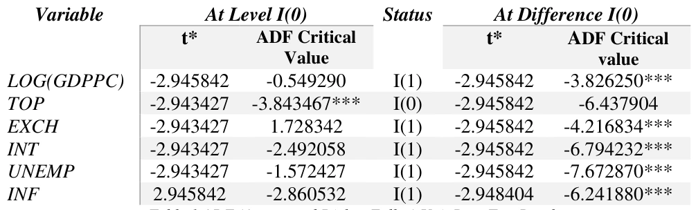
Table 1 presents the outcomes of the unit root test. The ADF (augmented Dickey-Fuller) test is used to establish the order of integration of the variables, with the null hypothesis being 𝐻𝑂: = 𝛽 = 0 (i.e. 𝛽 has a unit root) and the alternative hypothesis is 𝐻1: 𝛽 < 0 are implemented. The outcome is shown in table 1 above for both the level and differenced factors. To determine the presence of unit roots and the sequence of integration in all the variables, the stationarity tests were first carried out in levels and then in first difference. Results of the ADF stationarity tests for each variable show that for GDP per capita, exchange rate, interest rate, unemployment rate, and inflation rate data series at level, the test did not successfully reject the presence of unit root, indicating that these variables are non-stationary at levels while trade openness is stationary at level.
5.2. Co-integration Analysis
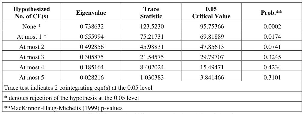
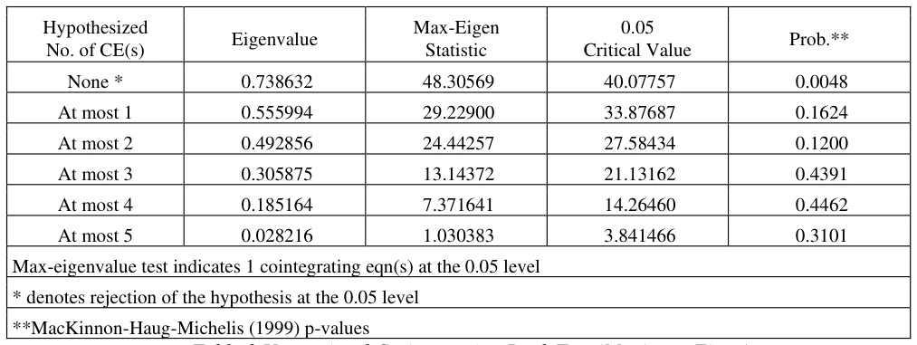
The Johansen Co-integration test is carried out to establish the existence of a long-run relationship between the variables. The tables 2a and 2b below report the test result that was produced using the Johansen co-integration technique. According to the test results, the unrestricted trace rank test (maximum Eigenvalue) suggests the existence of two integrating vectors in the model and the unrestricted co-integration rank test (maximum Eigen-value) suggests the existence of one co-integrating vector. The conclusion therefore implies that there is a long-run relationship between the variables.
0.05 Critical Value Prob.**
Accessible table text
| Hypothesized No. of CE(s) | Eigenvalue | Trace Statistic | 0.05 Critical Value | Prob.** |
|---|---|---|---|---|
| None * | 0.738632 | 123.5230 | 95.75366 | 0.0002 |
| At most 1 * | 0.555994 | 75.21731 | 69.81889 | 0.0174 |
| At most 2 | 0.492856 | 45.98831 | 47.85613 | 0.0741 |
| At most 3 | 0.305875 | 21.54575 | 29.79707 | 0.3245 |
| At most 4 | 0.185164 | 8.402024 | 15.49471 | 0.4234 |
| At most 5 | 0.028216 | 1.030383 | 3.841466 | 0.3101 |
| Trace test indicates 2 cointegrating eqn(s) at the 0.05 level | — | — | — | — |
| * denotes rejection of the hypothesis at the 0.05 level | — | — | — | — |
| **MacKinnon-Haug-Michelis (1999) p-values | — | — | — | — |
Accessible table text
| Hypothesized No. of CE(s) | Eigenvalue | Max-Eigen Statistic | 0.05 Critical Value | Prob.** |
|---|---|---|---|---|
| None * | 0.738632 | 48.30569 | 40.07757 | 0.0048 |
| At most 1 | 0.555994 | 29.22900 | 33.87687 | 0.1624 |
| At most 2 | 0.492856 | 24.44257 | 27.58434 | 0.1200 |
| At most 3 | 0.305875 | 13.14372 | 21.13162 | 0.4391 |
| At most 4 | 0.185164 | 7.371641 | 14.26460 | 0.4462 |
| At most 5 | 0.028216 | 1.030383 | 3.841466 | 0.3101 |
| Max-eigenvalue test indicates 1 cointegrating eqn(s) at the 0.05 level | — | — | — | — |
| * denotes rejection of the hypothesis at the 0.05 level | — | — | — | — |
| **MacKinnon-Haug-Michelis (1999) p-values | — | — | — | — |
5.3. Auto-Regressive Distributed Lag (ARDL)

Accessible table text
| — | Computed Wald F-statistic: 5.931370; K = 5 | — | — | — | — | — | — | — |
|---|---|---|---|---|---|---|---|---|
| — | Bounds Level | — | — | Lower Bound | — | — | Upper Bound | — |
| — | 1% critical bounds value | — | 3.41 4.68 | — | — | — | — | — |
| — | 5% critical bounds value | — | — | 2.62 | — | — | 3.79 | — |
| — | 10% critical bounds value | — | 2.26 3.35 | — | — | — | — | — |
The result of the co-integration test, based on the ARDL bound testing approach, is presented in Table 3. The result revealed that computed F-Statistics for Wald test was
5.931370. The value exceeds both the upper bounds and lower bounds critical values for all level of significance. This indeed implies that trade liberalization, selected independent variables and real GDPPC are bound by a long run relationship in Nigeria which means that the variables included in the model shared long-run relationships among themselves.
The short-run and long-run ARDL results for the effect of trade liberalization on poverty in Nigeria are presented in Table 4 and 5 below.
Accessible table text
| Variable | Coefficient | Std. Error | t-Statistic | Prob. |
|---|---|---|---|---|
| TOP | -0.730176 | 0.390410 | -1.870279 | 0.0727* |
| EXCH | 0.002039 | 0.000837 | 2.435867 | 0.0220** |
| INT | 0.022504 | 0.011990 | 1.876816 | 0.0718* |
| UNEMP | 0.032059 | 0.015779 | 2.031788 | 0.0525* |
| INF | -0.005803 | 0.003022 | -1.920024 | 0.0659* |
| C | 7.147270 | 0.258252 | 27.675537 | 0.0000 |
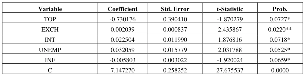
Table 4 represents the long-run impact of the variables on poverty rate in Nigeria. The analysis shows that all the variables are statistically significant in determining poverty rate in Nigeria in the long-run. Trade openness, interest rate, unemployment rate and inflation rate are statistically significant at 10% level of significance while exchange rate is statistically significant at 5% level of significance. The coefficient of the variable shows that trade openness and inflation rate are negatively related to poverty rate Nigeria while exchange rate, interest rate and unemployment rate are positively related to poverty rate in Nigeria. The implication of the coefficient value is that a percentage increase in each of trade openness and inflation rate will reduce poverty rate in Nigeria in the long-run by 0.73% and 0.0058% respectively. Also, a percentage increase in each of exchange rate, interest rate and unemployment rate will increase poverty rate in Nigeria in the long-run by 0.0020%, 0.0225% and 0.032% respectively.
According to studies by Hameed & Nazir (2009), who found that economic globalization could eventually lessen poverty, trade openness has a detrimental long-term effect. However, a country's economic system's potential to gain from economic globalization also depended on its domestic macroeconomic policy, market structure, early economic state, institutional quality, and degree of political stability. The similar conclusion was reached by Ozcan & Kar (2016), Okungbowa & Eburajolo (2014), and Oyewale & Amusat (2013). According to the predicted outcome, trade will benefit the poor in the long run. Additionally, it necessitates additional work in order for the poor to benefit from global trade. It will become a reality once trade policy enables and safeguards the micro-economic agent to enable global trade competition.
Accessible table text
| D(TOP) | -0.126281 | 0.060686 | -2.080872 | 0.0474 |
|---|---|---|---|---|
| D(EXCH) | -0.000411 | 0.000488 | -0.841167 | 0.4079 |
| D(EXCH(-1)) | -0.001584 | 0.000514 | -3.078490 | 0.0049 |
| D(INT) | 0.003892 | 0.001322 | 2.944269 | 0.0067 |
| D(UNEMP) | -0.001380 | 0.003125 | -0.441581 | 0.6624 |
| D(INF) | -0.001004 | 0.000392 | -2.560799 | 0.0166 |
| ECT(-1) | -0.172945 | 0.055229 | -3.131447 | 0.0043 |
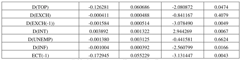
Table 5 above represents the short-run impact of the variables on poverty rate in Nigeria. The analysis shows that in the short-run, trade openness, exchange rate at a year lag, interest rate, and inflation rate are statistically in determining poverty rate in Nigeria at 5%, 1%, 1% and 1% level of significance respectively while exchange rate and unemployment rate are statistically insignificant in determining poverty rate in Nigeria in the short-run. The coefficient values show that trade openness, exchange rate, exchange rate at 1-year lag, unemployment rate and inflation rate are negatively related to poverty rate in Nigeria in the short run while interest rate is positively related to poverty rate in Nigeria in the short-run. A percentage increase in each of trade openness, exchange rate, exchange rate at 1-year lag, unemployment rate and inflation rate in the short-run will reduce poverty rate in Nigeria by 0.126%, 0.0004%, 0.0016%, 0.0014% and 0.001% respectively. Also, a percentage increase in interest rate in Nigeria in the short-run will increase poverty rate in Nigeria by 0.0039%.
The error correction term (ECT), which will be used to assess how the variables will converge to equilibrium, must meet the benchmark that it be negative and significant at any level of significance. As a result, the coefficient of the error correction term (ECT) showed that the annual correction for the 17.29 percent variation in the poverty rate from the long-run equilibrium. Additionally, the modified R-square of 0.985116 showed that the whole variation in the poverty rate can be explained by all the explanatory factors by around 98.5 percent.
5.4. Pairwise Granger Causality Result
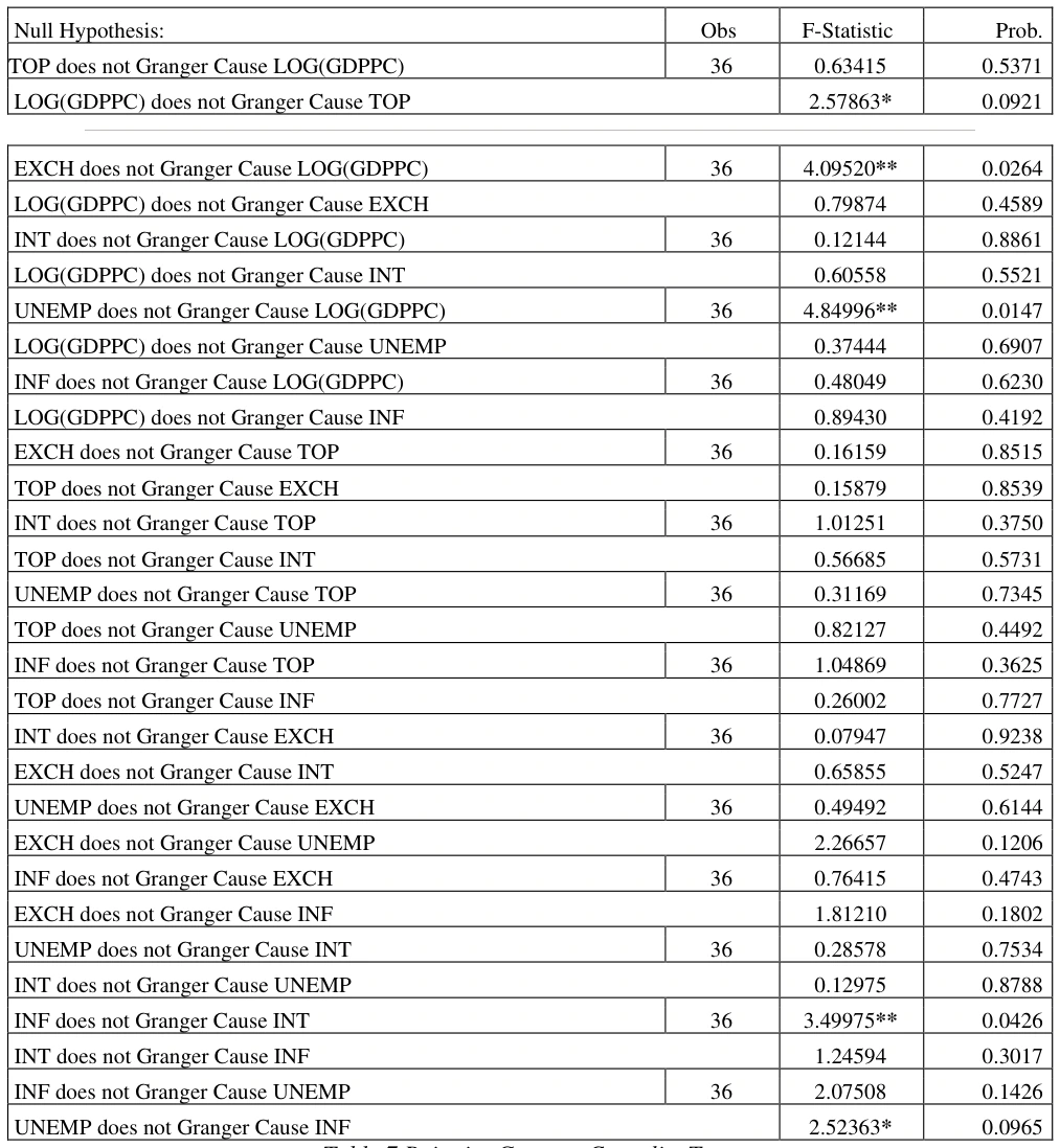
The Granger causality technique is used in this part to evaluate the causal link structures between the study's variables. A statistical hypothesis test for detecting if one time series is helpful for forecasting another is the Granger causality test. The hypothesis would be rejected at the level if the probability value is less than any P-Value level.
Accessible table text
| Null Hypothesis: | Obs | F-Statistic | Prob. |
|---|---|---|---|
| TOP does not Granger Cause LOG(GDPPC) | 36 | 0.63415 | 0.5371 |
| LOG(GDPPC) does not Granger Cause TOP | — | 2.57863* | 0.0921 |
| EXCH does not Granger Cause LOG(GDPPC) | 36 | 4.09520** | 0.0264 |
| LOG(GDPPC) does not Granger Cause EXCH | — | 0.79874 | 0.4589 |
| INT does not Granger Cause LOG(GDPPC) | 36 | 0.12144 | 0.8861 |
| LOG(GDPPC) does not Granger Cause INT | — | 0.60558 | 0.5521 |
| UNEMP does not Granger Cause LOG(GDPPC) | 36 | 4.84996** | 0.0147 |
| LOG(GDPPC) does not Granger Cause UNEMP | — | 0.37444 | 0.6907 |
| INF does not Granger Cause LOG(GDPPC) | 36 | 0.48049 | 0.6230 |
| LOG(GDPPC) does not Granger Cause INF | — | 0.89430 | 0.4192 |
| EXCH does not Granger Cause TOP | 36 | 0.16159 | 0.8515 |
| TOP does not Granger Cause EXCH | — | 0.15879 | 0.8539 |
| INT does not Granger Cause TOP | 36 | 1.01251 | 0.3750 |
| TOP does not Granger Cause INT | — | 0.56685 | 0.5731 |
| UNEMP does not Granger Cause TOP | 36 | 0.31169 | 0.7345 |
| TOP does not Granger Cause UNEMP | — | 0.82127 | 0.4492 |
| INF does not Granger Cause TOP | 36 | 1.04869 | 0.3625 |
| TOP does not Granger Cause INF | — | 0.26002 | 0.7727 |
| INT does not Granger Cause EXCH | 36 | 0.07947 | 0.9238 |
| EXCH does not Granger Cause INT | — | 0.65855 | 0.5247 |
| UNEMP does not Granger Cause EXCH | 36 | 0.49492 | 0.6144 |
| EXCH does not Granger Cause UNEMP | — | 2.26657 | 0.1206 |
| INF does not Granger Cause EXCH | 36 | 0.76415 | 0.4743 |
| EXCH does not Granger Cause INF | — | 1.81210 | 0.1802 |
| UNEMP does not Granger Cause INT | 36 | 0.28578 | 0.7534 |
| INT does not Granger Cause UNEMP | — | 0.12975 | 0.8788 |
| INF does not Granger Cause INT | 36 | 3.49975** | 0.0426 |
| INT does not Granger Cause INF | — | 1.24594 | 0.3017 |
| INF does not Granger Cause UNEMP | 36 | 2.07508 | 0.1426 |
| UNEMP does not Granger Cause INF | — | 2.52363* | 0.0965 |
Table 6 above represents the Pairwise Granger Causality Tests of the variables in this study. The result shows that there is a uni-directional causal relationship between GDP per capita and trade openness as only GDP per capital granger caused trade openness. The causal relationship between exchange rate and GDP per capita is uni-directional as only exchange rate granger caused GDP per capita. The causal relationship between interest rate and GDP per capita is non-directional as none of the variables granger caused each other. The causal relationship between unemployment rate and GDP per capita is uni-directional as only unemployment rate granger caused GDP per capita. The causal relationship between inflation rate and GDP per capita is non-directional as none of the variables granger caused each other.
The causal relationship between exchange rate and trade openness is non-directional as none of the variables granger caused each other. The causal relationship between interest rate and trade openness is non-directional as none of the variables granger caused each other. The causal relationship between unemployment rate and trade openness is nondirectional as none of the variables granger caused each other. The causal relationship between inflation rate and trade openness is non-directional as none of the variables granger caused each other. The causal relationship between interest rate and exchange rate is non-directional as none of the variables granger caused each other. The causal relationship between unemployment rate and exchange rate is non-directional as none of the variables granger caused each other. The causal relationship between inflation rate and exchange is non-directional as none of the variables granger caused each other. The causal relationship between unemployment rate and interest rate is non-directional as none of the variables granger caused each other. The causal relationship between inflation rate and interest rate is uni-directional as only inflation rate granger caused interest rate. The causal relationship between inflation rate and unemployment rate is uni-directional as only unemployment rate granger caused inflation rate.
6. Conclusion
The outcome demonstrated that trade is statistically important in determining Nigeria's poverty rate over the long run and short run. The variable's coefficient demonstrates that trade has both a short-run and long-run negative relationship with Nigeria's poverty rate. According to the predicted outcome, trade will benefit the poor in the long run. Additionally, it necessitates additional work in order for the poor to benefit from global trade. It will become a reality once trade policy enables and safeguards the microeconomic agent to enable global trade competition.
Conclusively, both in the short and long run, international trade does have a substantial impact on poverty. Therefore, the creation of a fair-trade system is necessary in order to eliminate poverty through international trade. Those nations that implemented sensible economic policies and were open to trade have gained, while those that did not have to pay a price. Therefore, every nation must try to implement policies that can keep up with the realities of the world's economies' growing integration.
Recommendation
On the basis of the study's findings, suggestions are given to promote trade and lower the rate of poverty in Nigeria. The results of this analysis indicate that in order to save its domestic market, Nigeria may pursue a policy of restrictive trade liberalization. In contrast, the government should encourage the import of technology to advance domestic industry and adopt a soft trade liberalization policy that is based on the elimination or reduction of barriers to international trade in technology. For the import of agricultural and industrial apparatus, equipment, and technology, this involves the elimination or reduction of both tariff (duties and surcharges) and non-tariff impediments (such as licensing restrictions, quotas, and other requirements). In order for the domestic industry to prosper, wages and employment levels rise. This would improve Nigeria's economic development through lowering poverty, increasing GDP per capita, and other positive effects.
Data Availability
The datasets collected and/ or analysed during the current study are available from the corresponding author on request. The corresponding authors has full access to the data in the study and takes responsibility for the integrity of the data and the accuracy of the data analysed.