 Journal of Global Trade, Ethics and Law
1. Introduction
In the last 30 years, there have been four major surprises for monetary theory and central bank policy.
First, after 1990 or so inflation began to respond less than before to short-run changes in unemployment (or other measures of economic slack.) (Bernanke 2022)
Not only did inflation respond less to economic slack measures but economic slack and inflation itself responded less to monetary stimulus. This led to persistent inflation shortfalls below central bank targets.
The main puzzle pertaining to inflation is aptly summed up by the title of this conference: “What’s (not) up with inflation?” Inflation hasn’t moved up through an expansion that now ranks as the nation’s longest on record. (Yellen 2019)
This period also saw a second surprise evolution in the nature of business cycles.
From the 1950’s to the 1980’s , recessions typically followed fed tightening that had been spurred by too high inflation...[S]ince 1990 , ...financial disruptions have played an increasingly important role in economic downturns. (Bernanke 2022)
Financial bubbles and cyclical disruptions became increasingly prevalent, but, in a third surprise, inflation resisted both upwards and downwards pressure.
During my time as chair, ...forecasters ...were nevertheless surprised by how modestly inflation declined following the financial crisis. (Bernanke 2022)
Resilient inflation despite extreme cyclical pressures also characterized the later pandemic crisis, which then produced the fourth major surprise – the extent and duration of the pandemic inflation unforeseen by almost all forecasters, even those expecting an uptick.
A consequence of these surprises has been the inability of major central banks to attain their 2% inflation targets, illustrated in Figure 1.

This paper introduces a new framework for understanding inflation that explains these surprises, breaking inflation into three components:
The Natural Rate of Inflation. Each economy has an underlying inflation rate determined by non-monetary factors – the rate of population growth and an economy’s vitality as reflected in its natural rate of interest. The Natural Inflation Rate evolves slowly over decades and sets a minimal base level for inflation, around which other influences produce shorter-term oscillations. The Natural Inflation Rate explains the low-end resiliency of inflation.
Monetary Inflation. Virtually all variability of medium to long-term inflation (5 years plus) can be explained as a unique function of monetary aggregates. In contrast to the traditional Quantity Theory, this model is characterized by a geometric relationship between money and inflation, which explains the diminished responsiveness of inflation to monetary stimulus and a consequent increased financial component of business cycles.
Cyclical inflation. Shorter-term inflation factors range in influence from a few months up to three years. Fiscal balance is a policy-related cyclical factor as are non-policy influences such as external balances and demand shifts, although non-policy measures may relate closely to policy. Viewed from this paper’s framework, the pandemic inflation is the most prominent example of cyclical factors’ effect.
The next three sections of the paper describe each of these inflation components, starting with monetary inflation, which, because of its high explanatory power, helps identify and specify Natural Inflation and cyclical factors. The paper then examines real effects from the monetary model and economic risks identified with this analytical framework.
2. The Money Value Monetary Inflation Model
This paper’s monetary model flips the problem of estimating and forecasting inflation on its head. Instead of measuring an ever-varying, large, representative, diverse crosssection of market prices for goods and services throughout a complex advanced economy, then estimating future movements in this sample to project general inflation, the Money Value model estimates just one price, the unit value of a currency, then projects general inflation from that basis.
A simple Econ 1 example illustrates the premise. Take an economy with 10 widgets and $100 suggesting a price, everything being equal and neutral, of $10/widget. Should the money stock be $200, the presumed price is $20/widget, 100% inflation.
The unit value of a currency, if the outstanding money stock can be ascribed a value of C, is expressed as a simple function of this constant value and the money stock as follows:

where
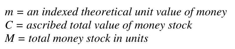
Since there is no generally accepted, identifiable quantitative basis for ascribing an absolute value to the money stock, for example a quantity of widgets the money stock is worth, we must settle for describing the relative value of money in terms of some reference point t0.
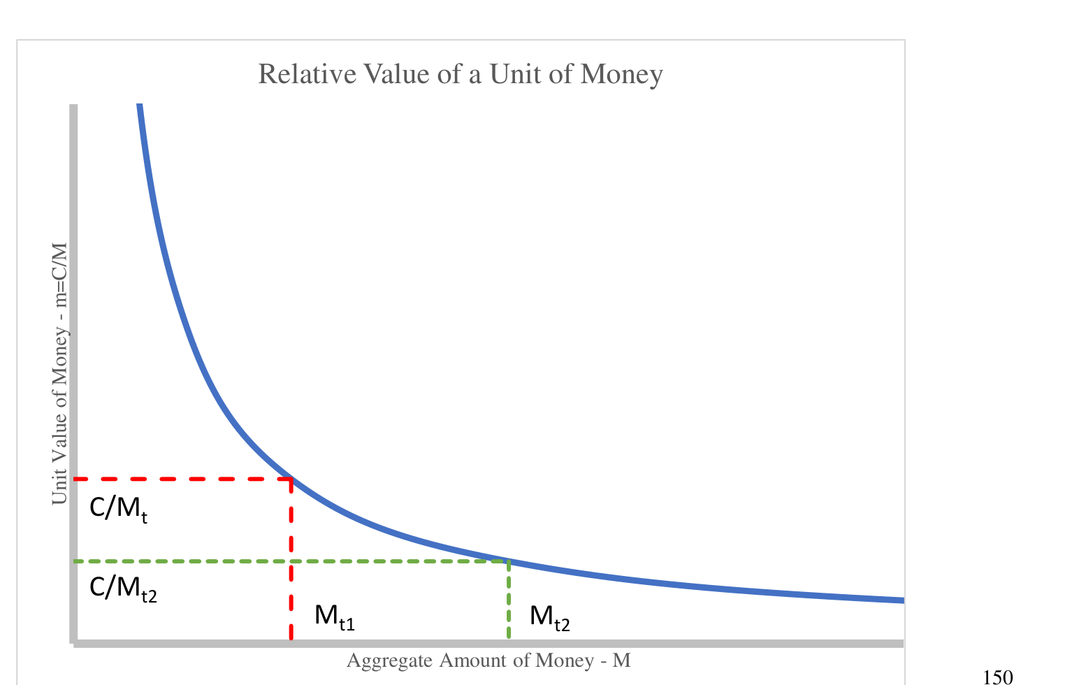
The change in unit value of money is thus:

From Equation 3, we can see as the difference between Mt1 and Mt2 shrinks:

The same result is obtained by differentiating Equation 2:

Inflation, increases in the price level, is the inverse of decreases in the unit value of money. Including a term for possible non-monetary causes, inflation is represented as:

where π = total inflation πM = inflation due to monetary causes πr = inflation due to non-monetary or residual causes If we view residual inflation as attributable to influences such as population growth or other factors, we may consider them functions of time. The price level can then be represented by integrating Equation 6 as follows:

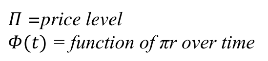
The Money Value formula in Equation 5 relies solely upon a constant and the level of a monetary aggregate. The model may be thought of as similar to the Quantity Theory; each explains inflation directly as a function of money, but the Money Value formula has an inherent non-linear relationship between money stock and prices while the Quantity Theory implies a proportionally linear relationship under typical assumptions about velocity and real growth. In utilizing the concept of velocity, or turnover, of money, the Quantity Theory is based upon the function of money as a means of exchange. The Money Value model relies upon money’s function as a store of value, which is represented by credit and thus may incorporate aggregates such as central bank or banking system assets in addition to customary money measures.
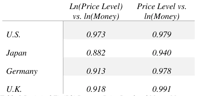
Equation 7’s relationship between price level and the log of money also reflects the non-linear relationship posited by the Money Value model. Figures 3a-d depict this relationship for some major advanced economies.
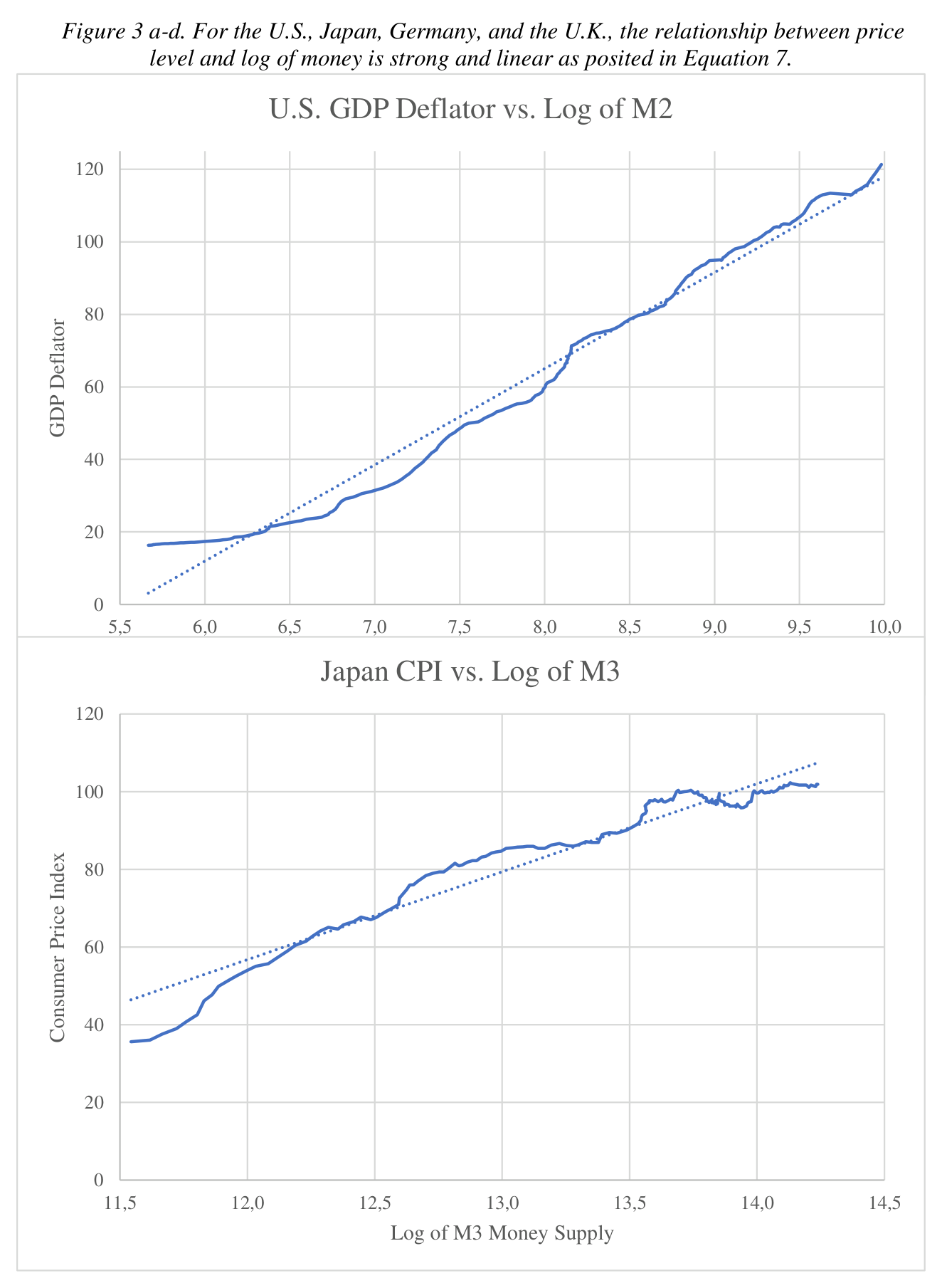

In all cases, the log of money appears linear with the price level, as expressed in Equation 7. The statistical fit for these various measures appears in Table 1.
Accessible table text
| — | — | — | — | Ln(Price Level) | — | — | Price Level vs. | — |
|---|---|---|---|---|---|---|---|---|
| — | — | — | — | vs. ln(Money) | — | — | ln(Money) | — |
| — | U.S. | — | — | 0.973 | — | — | 0.979 | — |
| — | Japan | — | 0.882 0.940 | — | — | — | — | — |
| — | Germany | — | — | 0.913 | — | — | 0.978 | — |
| — | U.K. | — | 0.918 0.991 | — | — | — | — | — |
For these economies, Equation 7’s fit between price level and the log of money is higher than what might more customarily be expected, the log of prices against the log of money.
The original Equation 1 also can be examined in Figures 4a-d to evaluate whether real world data conforms to the hyperbolic relationship between the value and amount of money suggested in Figure 2. For each of the advanced economies examined, the unit currency value calculated from an inflation index is compared with a monetary aggregate.
Figure 4 a-d. The hyperbolic relationship between the value and amount of money depicted
in Figure 2 applies to each of the U.S., Japan, Germany, and U.K.
U.S. GDP Deflator Dollar Unit Value vs. M2
$7,50
$6,50
Unit Value of Dollar 4Q2021 = $1.00
$5,50
$4,50
$3,50
$2,50
$1,50
$0,50
$0 $5.000 $10.000 $15.000 $20.000 $25.000
M2 Money Supply ($000,000)
Japan CPI Unit Value of Yen vs. M3
¥3,00
Unit Value of Yen 4Q2021 = ¥1.00
¥2,50
¥2,00
¥1,50
¥1,00
¥0,50
¥0 ¥200.000 ¥400.000 ¥600.000 ¥800.000¥1.000.000¥1.200.000¥1.400.000¥1.600.000¥1.800.000
M3 Money Supply (¥00,000)
Germany CPI Unit Value vs. M1
€5,50
€5,00
€4,50
Unit Value of Euro 4Q2021 = €1.00
€4,00
€3,50
€3,00
€2,50
€2,00
€1,50
€1,00
€0,50
€0 €3.000.000 €6.000.000 €9.000.000 €12.000.000
M1 Money Supply (€000)
U.K. GDP Deflator Pound Unit Value vs. Broad Money
£30,00
£25,00
Unit Value of Pound 4Q2021 = £1.00
£20,00
£15,00
£10,00
£5,00
£0,00
£0 £500.000 £1.000.000 £1.500.000 £2.000.000 £2.500.000
Broad Money Supply
Figure 2’s hyperbolic relationship between the amount of money and its value holds for each economy in Figure 4.
3. Inflation Elasticity
Another attribute of the Money Value model is that an elasticity for inflation can be derived from Equation 6 as follows:

The more the absolute level of money in an economy grows from its reference point, Mto, the greater the percentage increase in money must be to effect a given level of inflation. Inflation Elasticity becomes increasingly inelastic. This is consistent with inflation target shortfalls in advanced economies prior to the pandemic. The more a currency has been inflated, the more difficult it is to further inflate it, unless launching into hyperinflation, which is extremely difficult, albeit possible in this framework. This is precisely the surprise from the 1990’s identified in the introduction by Dr. Bernanke.
4. Empirical Evaluation
The Money Value model can be tested empirically with lags of monetary aggregates regressed against forward inflation. Detailed development of regression parameters appears in Appendix A. In this section, the following formula will be tested:

where
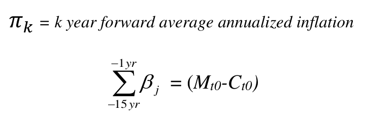
Table 2 contains regression statistics for lagged values of U.S. M2 against forward inflation measured by the core PCE inflation index.

The Money Value formula provides an exceptionally strong statistical explanation of forward inflation in the U.S. Table 3 provides a similar comparison for 10 year forward inflation in the selected advanced economies.
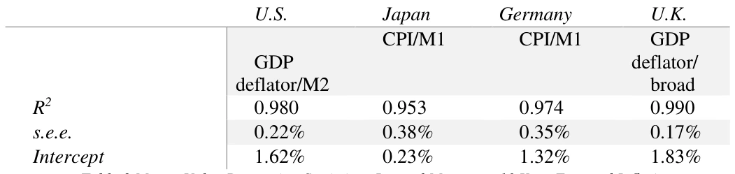
The Money Value formula provides a strong explanation of forward inflation for these advanced economies.
5. The Natural Rate of Inflation
Regression results with the Money Value Formula invariably produce a significant constant term in the range of 1.00-2.00% for the U.S. with a broader range for international analyses. The formula thus explains virtually all long-term inflation variability, but the base level of inflation, represented by the intercept, may have an alternative, non-monetary cause. Harold Hotelling’s (1931) famous theory that resource prices appreciate at the interest rate is a possible non-monetary explanation of price level changes. Several papers also explore shifting demographics as a potential influence on prices. These two factors will be analysed in combination with the Money Value Formula to evaluate whether they have additional, significant effects on inflation and account for the base or Natural Rate of Inflation represented by the Money Value regression intercepts.
5.1. Hotelling and Prices
Hotelling (1931) found that commodity production rates should be consistent with pricing that appreciates with the rate of interest. Empirical tests such as described by Hart and Spiro (2011) and Livernois (2009) have generally not confirmed a Hotelling effect for commodities. Testing in conjunction with the Money Value Formula can highlight a possible Hotelling effect by accounting for the variability of inflation from monetary factors.
Further, while Hotelling restricted his focus to finite depletable commodities, it is not clear such effect is thus limited. For example, Hotelling’s basic equation is

where
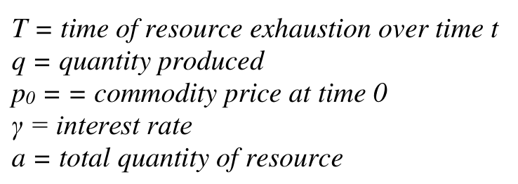
Perhaps a similar dynamic might apply to a worker’s labours. T could be their retirement and the interest rate might correspond to productivity increases. Accordingly, the Hotelling effect will be tested with the Money Value Formula against broad inflation indices as well labour prices.
5.2. Population Growth and Prices
Recently, several studies have evaluated the relationship between inflation and population growth or demographic shifts, which are a function of population growth. Bullard et al (2012), Anderson et al (2014), Juselius and Takáts (2015), and Bobeica et al (2017) all have found a positive relationship between population growth and inflation. These works used sophisticated demographic analyses to focus on the relationship. For inclusion with the Money Value Formula, just the population growth rate is incorporated as an additional variable. This may be considered a “naïve” test of the population effect justified that demand rises proportionately to population and price elasticity is around one.
5.3. Empirical Analysis of Hotelling and Population Growth
Price effects from Hotelling and population growth are evaluated for the U.S. from 1952 to 2012 with a linear regression of Formula values using M2 lagged sequentially for fifteen years and with interest rates and population growth as separate variables. Both real T-bill rates and a proxy for the natural rate of interest described in Appendix B are used for interest rates. The natural rate proxy is closely related to potential economic growth.
5.3.1. Time Series Regressions Test with Money Value Formula
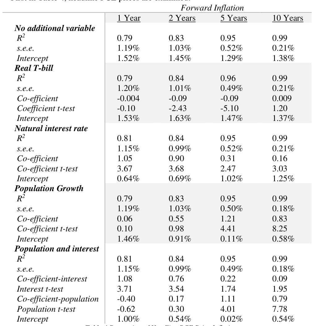
As in the previous section’s analyses, the Money Value Formula explains a very large amount of the variability of headline PCE prices, up to 99% at the 10-year horizon. Actual market interest rates do not display a Hotelling effect for headline PCE, but the natural rate of interest does. The natural interest rate co-efficient is around one, significant, and reduces the intercept, explaining a portion of non-monetary effects upon prices. The effect fades over time, although forward natural interest rates do maintain a high level of significance if included as a variable. Alternative natural rate measures such as Laubach-Williams (2015) also have a significant correlation with different co-efficients. This analysis suggests a Hotelling effect exists in broad inflation indices. Population growth appears to have no initial effect but a strong long-term effect, whether evaluated independently or with the natural interest rate.
Table 5 performs a similar analysis on core PCE prices using just the natural rate proxy as an interest rate.
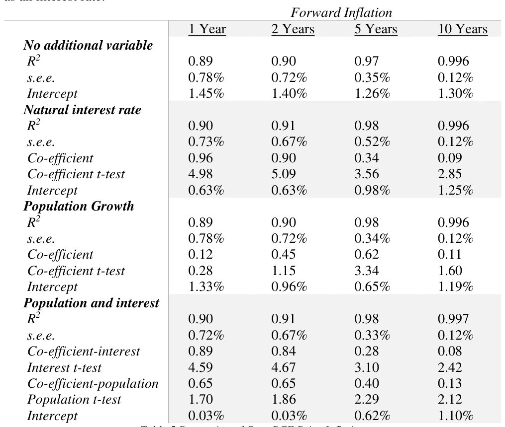
As with headline figures, the Money Value Formula explains a high amount of core PCE price variability. Again, the natural interest co-efficient is significant and around one initially, fading over time, and reduces the intercept, suggesting an apparent Hotelling effect. Population growth is closer to significance initially with the less volatile core measure but appears to have less long-term impact. When both natural rate and population growth are analysed together, the intercept term, which had been highly significant, all but vanishes, so these variables may account for the observed non-monetary price effects.
Earlier, it was proposed the basic Hotelling formula might apply to labour, with individuals having a finite career as does each commodity deposit. Table 6 tests Money Value, Hotelling, and population growth against hourly wages for the U.S.

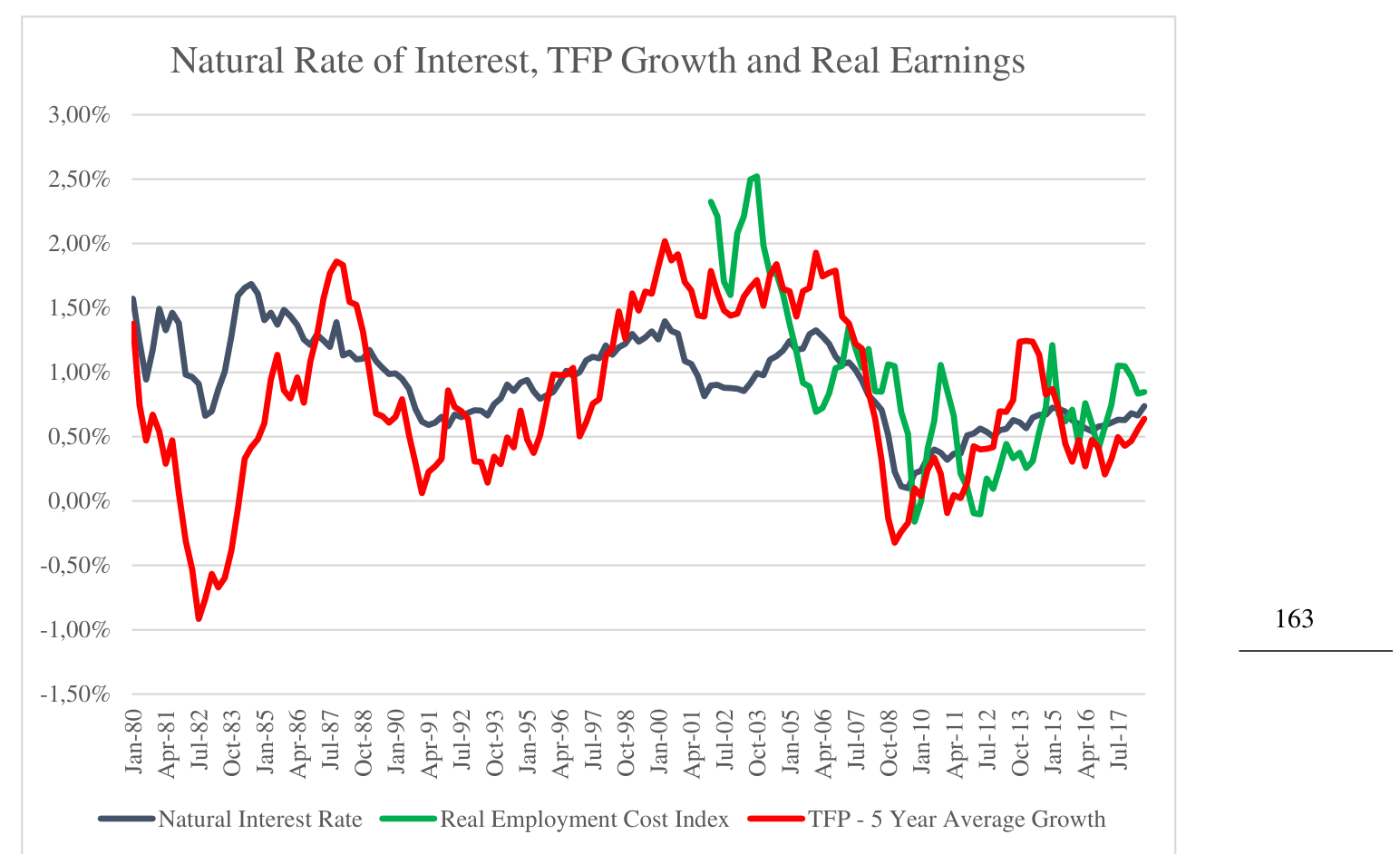
As with the broader inflation indices, there is a strong correlation with the Money Value Formula and an apparent significant but short-lived Hotelling effect on U.S. wages. Population also has a strong correlation that increases with time. It might be expected that population growth has an inverse relationship with wage inflation – more people, more workers, lower compensation, but the general positive correlation between population growth and inflation also holds with wages. The natural interest Hotelling correlation with wages may be due to convergences between productivity measures and the natural interest rate proxy as illustrated in Figure 5.
5.3.2. Cross-Sectional Test with OECD Economies
The geometric decline of inflation sensitivity to monetary stimulus evident in the Money Value Formula reached a point in the U.S. around 1995, shown in Figure 4a, where incremental monetary stimulus has minimal direct effect on pre-pandemic inflation. Domestic measures of inflation may continue to be impacted by factors such as fiscal measures, but the unit value of a currency associated with the Formula is virtually unchanged. Other advanced economies also had low, stable pre-pandemic inflation rates that appeared resistant to monetary stimulus. These economies with little or no inflation variability from monetary sources may be useful for testing the influence on prices of non-monetary factors examined in this paper.
Inflation, measured by the GDP deflator for consistency across economies, is compared to population growth and the natural rate of interest for OECD economies for 2009-2017, prior to pandemic distortions, in cross-section regressions in Table 7.
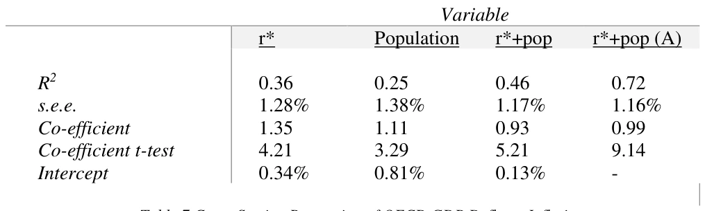
Both the natural rate of interest and population growth are significant regressed against inflation, all co-efficients are near one, and, combined, they explain almost all the level of inflation (no residual intercept) and much of its variation from country to country during the last ten years.

The average sum of population growth and natural interest is virtually identical to average inflation for OECD economies over 2009-2017. Correlation between inflation and the sum of natural interest and population growth is illustrated in Figure 6.
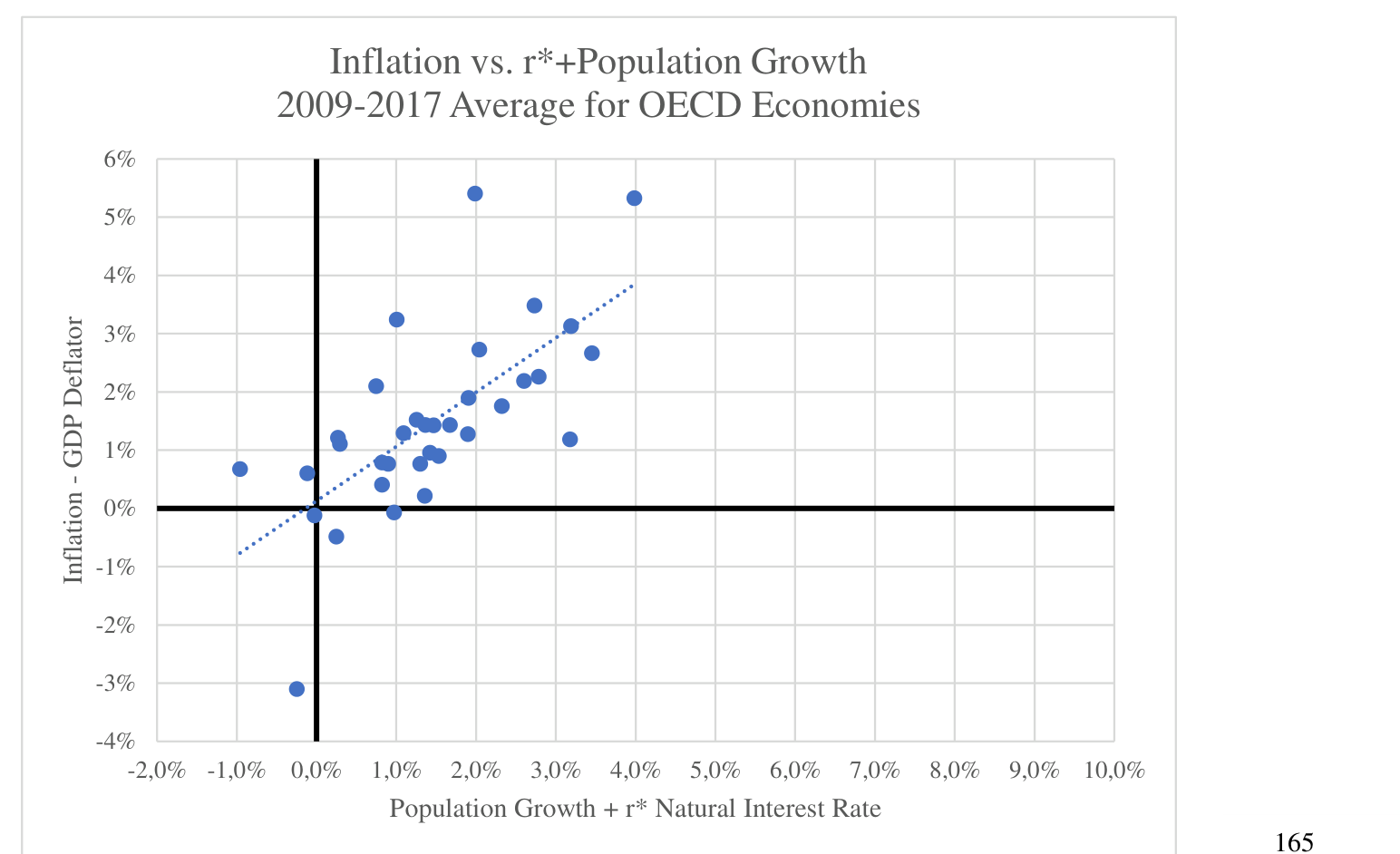
Figure 6 illustrates the regressions in Table 7 demonstrating the Natural Rate of Inflation in Money Value analysis can be entirely attributed to population growth and the natural rate of interest.
6. Cyclical Inflation
The long-term orientation of both the Natural Inflation Rate and the Money Value monetary model depict inflation as a smooth descending path, smooth because of multiyear perspectives and descending because of the inelasticity of monetary inflation and the slowing growth and diminished vitality of the major economies analysed in this paper with consequent effect upon Natural Inflation.
Of course, in the short-term, there can be significant variation of inflation from its smooth long-term path. The pandemic inflation is a prominent example with short-term inflation forecasts experiencing their largest-ever errors. Unprecedented fiscal deficits and a supply/demand imbalance often are ascribed as causes of this variance. This section evaluates these shorter-term cyclical factors as determinants of inflation.
One approach for analysing short-term inflation determinants is to evaluate them as variances against longer-term inflation projections. In a comparison of historical forecasting accuracy in Appendix C, the most consistent models were the Money Value model, The Federal Reserve Board’s teal book, and a calculation of Inflation Expectations derived from financial market and inflation data by the Cleveland Federal Reserve. Forecast horizons ranged from one to ten years. The models could not be more different in their derivation. The Cleveland Fed model is a pure measure of inflation expectations with sophisticated adjustments compared with well-known TIPS market breakeven measures, while the Money Value model is a pure formulaic calculation based upon monetary aggregates. Nevertheless, as shown in Figure 7, these two measures have corresponded closely over their history and provide a similar long-term outlook today.
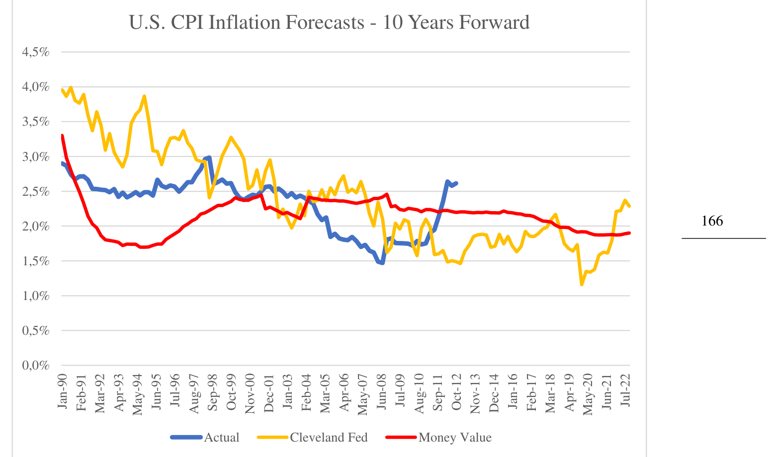
Interestingly, seemingly more difficult long-term inflation forecasts with each of these models are significantly more accurate than short-term forecasts.
6.1. Inflation and Fiscal Policy
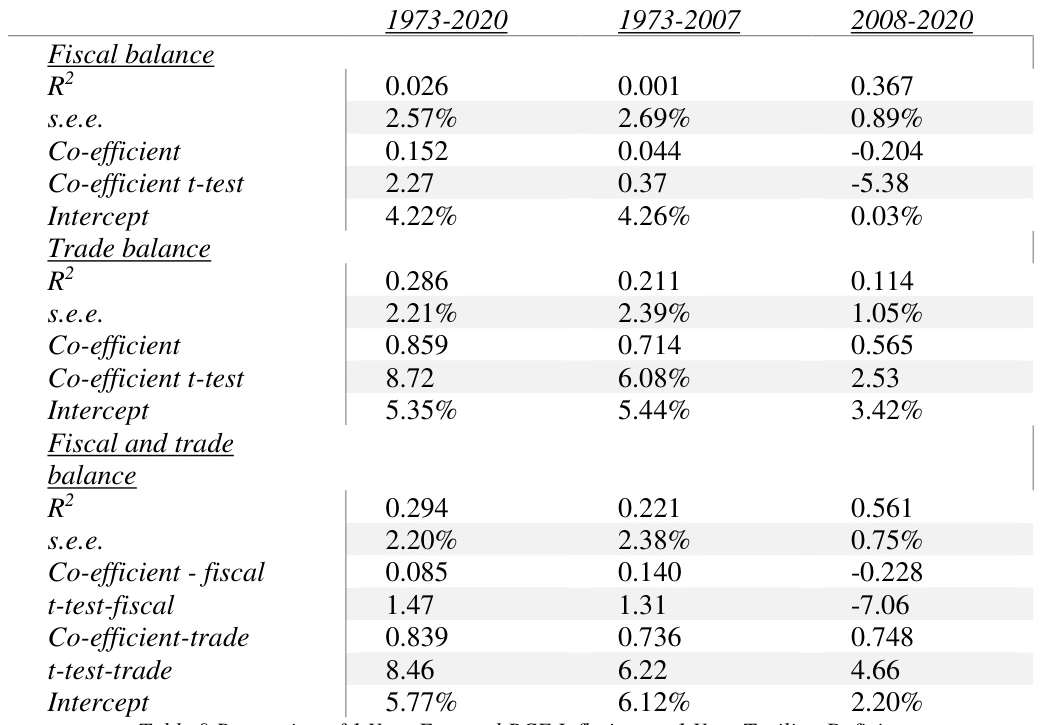
As analysed in Jorda (2022), it is reasonable to expect unprecedented loose U.S. fiscal policy contributed to inflation and inflation forecasting errors in the pandemic era. Standard economic principles suggest increased fiscal deficit expenditures should boost consumption and consequently inflation. Similarly, trade deficits could contribute to supply and lower inflation. Both government and external balances though are highly cyclical, so when regressed directly against forward inflation, the theoretically expected relationships can be reversed. Table 9 compares fiscal and trade balances in the modern, inelastic inflation era to short-term inflation, seen as most sensitive to supply/demand imbalances above.
Accessible table text
| — | — | — | — | 1973-2020 | — | — | 1973-2007 | — | — | 2008-2020 | — |
|---|---|---|---|---|---|---|---|---|---|---|---|
| — | Fiscal balance | — | — | — | — | — | — | — | — | — | — |
| — | R2 | — | 0.026 0.001 0.367 | — | — | — | — | — | — | — | — |
| — | s.e.e. | — | — | 2.57% | — | — | 2.69% | — | — | 0.89% | — |
| — | Co-efficient | — | 0.152 0.044 -0.204 | — | — | — | — | — | — | — | — |
| — | Co-efficient t-test | — | — | 2.27 | — | — | 0.37 | — | — | -5.38 | — |
| — | Intercept | — | 4.22% 4.26% 0.03% | — | — | — | — | — | — | — | — |
| — | Trade balance | — | — | — | — | — | — | — | — | — | — |
| — | R2 | — | 0.286 0.211 0.114 | — | — | — | — | — | — | — | — |
| — | s.e.e. | — | — | 2.21% | — | — | 2.39% | — | — | 1.05% | — |
| — | Co-efficient | — | 0.859 0.714 0.565 | — | — | — | — | — | — | — | — |
| — | Co-efficient t-test | — | — | 8.72 | — | — | 6.08% | — | — | 2.53 | — |
| — | Intercept | — | 5.35% 5.44% 3.42% | — | — | — | — | — | — | — | — |
| — | Fiscal and trade | — | — | — | — | — | — | — | — | — | — |
| — | balance | — | — | — | — | — | — | — | — | — | — |
| — | R2 | — | 0.294 0.221 0.561 | — | — | — | — | — | — | — | — |
| — | s.e.e. | — | — | 2.20% | — | — | 2.38% | — | — | 0.75% | — |
| — | Co-efficient - fiscal | — | 0.085 0.140 -0.228 | — | — | — | — | — | — | — | — |
| — | t-test-fiscal | — | — | 1.47 | — | — | 1.31 | — | — | -7.06 | — |
| — | Co-efficient-trade | — | 0.839 0.736 0.748 | — | — | — | — | — | — | — | — |
| — | t-test-trade | — | — | 8.46 | — | — | 6.22 | — | — | 4.66 | — |
| — | Intercept | — | 5.77% 6.12% 2.20% | — | — | — | — | — | — | — | — |
Since Bretton Woods, short-term inflation relationship with fiscal balance was inconsistent until the QE era. Since 2008, the fiscal-inflation relationship is strong, significant, and consistent with theoretical expectations. For the entire period, the trade balance has had a significant consistent relationship with short-term inflation.
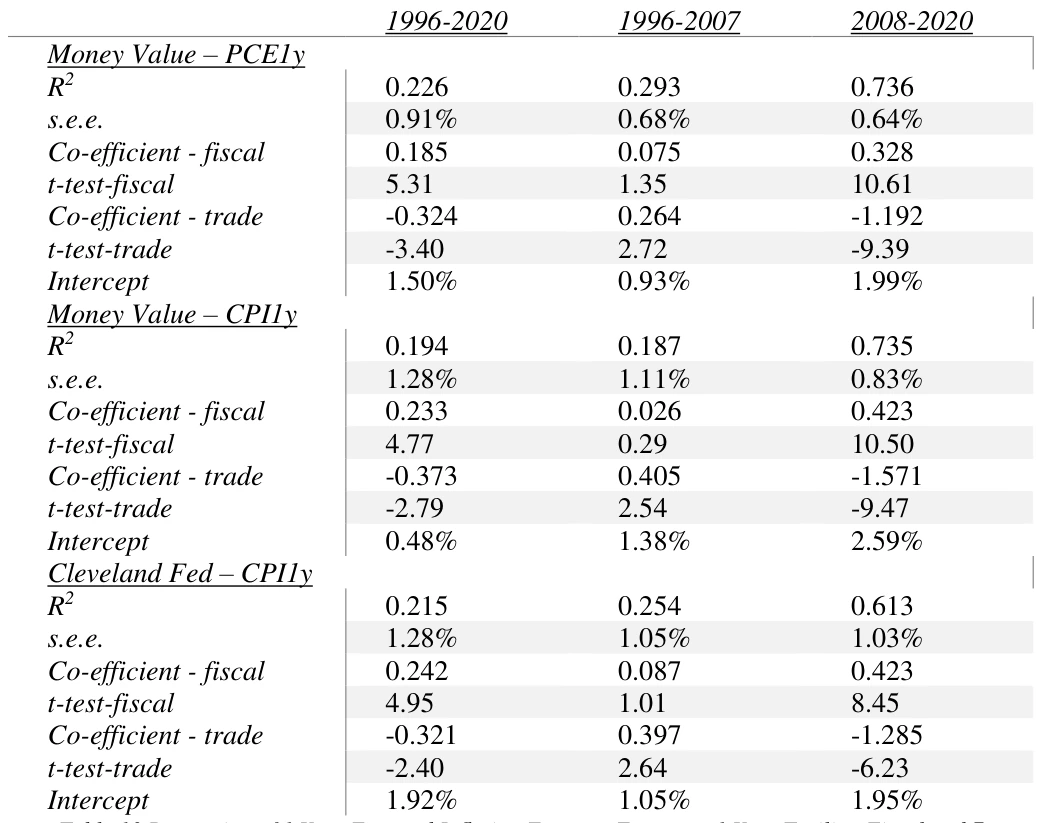
The significance of trade deficit effects on inflation increases with a lag. Table 10 compares lagged deficit data regressed against 1 year forward Money Value and Cleveland Fed expectations inflation forecast errors.
Accessible table text
| — | — | — | — | 1996-2020 | — | — | 1996-2007 | — | — | 2008-2020 | — |
|---|---|---|---|---|---|---|---|---|---|---|---|
| — | Money Value – PCE1y | — | — | — | — | — | — | — | — | — | — |
| — | R2 | — | 0.226 0.293 0.736 | — | — | — | — | — | — | — | — |
| — | s.e.e. | — | — | 0.91% | — | — | 0.68% | — | — | 0.64% | — |
| — | Co-efficient - fiscal | — | 0.185 0.075 0.328 | — | — | — | — | — | — | — | — |
| — | t-test-fiscal | — | — | 5.31 | — | — | 1.35 | — | — | 10.61 | — |
| — | Co-efficient - trade | — | -0.324 0.264 -1.192 | — | — | — | — | — | — | — | — |
| — | t-test-trade | — | — | -3.40 | — | — | 2.72 | — | — | -9.39 | — |
| — | Intercept | — | 1.50% 0.93% 1.99% | — | — | — | — | — | — | — | — |
| — | Money Value – CPI1y | — | — | — | — | — | — | — | — | — | — |
| — | R2 | — | 0.194 0.187 0.735 | — | — | — | — | — | — | — | — |
| — | s.e.e. | — | — | 1.28% | — | — | 1.11% | — | — | 0.83% | — |
| — | Co-efficient - fiscal | — | 0.233 0.026 0.423 | — | — | — | — | — | — | — | — |
| — | t-test-fiscal | — | — | 4.77 | — | — | 0.29 | — | — | 10.50 | — |
| — | Co-efficient - trade | — | -0.373 0.405 -1.571 | — | — | — | — | — | — | — | — |
| — | t-test-trade | — | — | -2.79 | — | — | 2.54 | — | — | -9.47 | — |
| — | Intercept | — | 0.48% 1.38% 2.59% | — | — | — | — | — | — | — | — |
| — | Cleveland Fed – CPI1y | — | — | — | — | — | — | — | — | — | — |
| — | R2 | — | 0.215 0.254 0.613 | — | — | — | — | — | — | — | — |
| — | s.e.e. | — | — | 1.28% | — | — | 1.05% | — | — | 1.03% | — |
| — | Co-efficient - fiscal | — | 0.242 0.087 0.423 | — | — | — | — | — | — | — | — |
| — | t-test-fiscal | — | — | 4.95 | — | — | 1.01 | — | — | 8.45 | — |
| — | Co-efficient - trade | — | -0.321 0.397 -1.285 | — | — | — | — | — | — | — | — |
| — | t-test-trade | — | — | -2.40 | — | — | 2.64 | — | — | -6.23 | — |
| — | Intercept | — | 1.92% 1.05% 1.95% | — | — | — | — | — | — | — | — |
Using forecast errors aligns relationships for inflation with trade and fiscal balances to their theoretical expected signs during the modern inflation era. Figure 8 displays the connection between forecast errors and combined government and external balances.
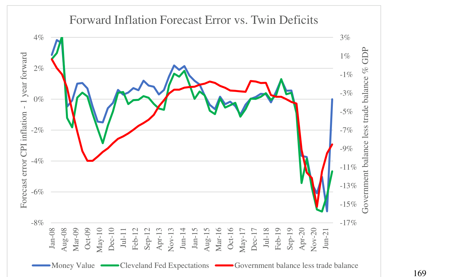
In the QE era since 2008, fiscal and trade balances explain the bulk of inflation variability and deviations from forecasts and expectations. The unprecedented pandemic deficits produced unprecedented forecasting and expectations errors.
6.2. Supply/Demand Imbalance and Inflation
A proxy representing the supply/demand imbalance can be derived from the ratio of personal consumption expenditures for goods to private inventories. This resembles the long-established concept of inventory/sales ratios, but personal consumption expenditures may be a better proxy for consumer demand. Figure 9 displays the relationship between PCE and CPI inflation measures with the supply/demand proxy ratio of goods PCE to inventories.
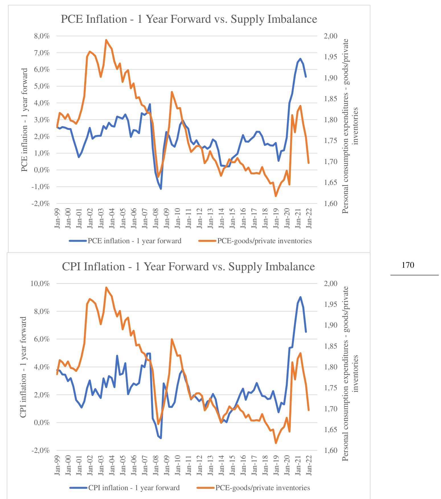
The supply/demand proxy appears highly correlated with future inflation, not just in the pandemic period but throughout the last two decades, especially during the Great Financial Crisis. Tables 11 and 12 contain regression statistics for the proxy against forward PCE and CPI inflation.

Accessible table text
| — | — | — | — | t-statistic | — | — | R2 | — |
|---|---|---|---|---|---|---|---|---|
| — | 1 year | — | — | 6.44 | — | — | 0.37 | — |
| — | 2 years | — | 10.12 0.59 | — | — | — | — | — |
| — | 5 years | — | — | 9.44 | — | — | 0.56 | — |
| — | 10 years | — | 4.90 0.32 | — | — | — | — | — |

Accessible table text
| — | — | — | — | t-statistic | — | — | R2 | — |
|---|---|---|---|---|---|---|---|---|
| — | 1 year | — | — | -3.80 | — | — | 0.17 | — |
| — | 2 years | — | 8.90 0.53 | — | — | — | — | — |
| — | 5 years | — | — | 8.30 | — | — | 0.50 | — |
| — | 10 years | — | 4.23 0.26 | — | — | — | — | — |
The supply/demand proxy explains over half the variability of forward inflation in the short to medium term. It has been a significant factor for the last two decades including not only the pandemic but the Great Financial Crisis and other sharp movements of inflation. Over the long-term, its impact fades significantly. Figure 9 suggests a return of inflation towards normal levels in 2023.
6.2.1. Supply/Demand Imbalance and Inflation Forecast Errors
The supply/demand proxy has a significant relationship with future inflation. Might it contribute to the inflation forecast errors recently so evident? Figure 10 depicts the relationship between the proxy and forecast errors included in this study. Unanticipated higher inflation produces a negative forecast error below the actual, so the proxy scale is inverted.
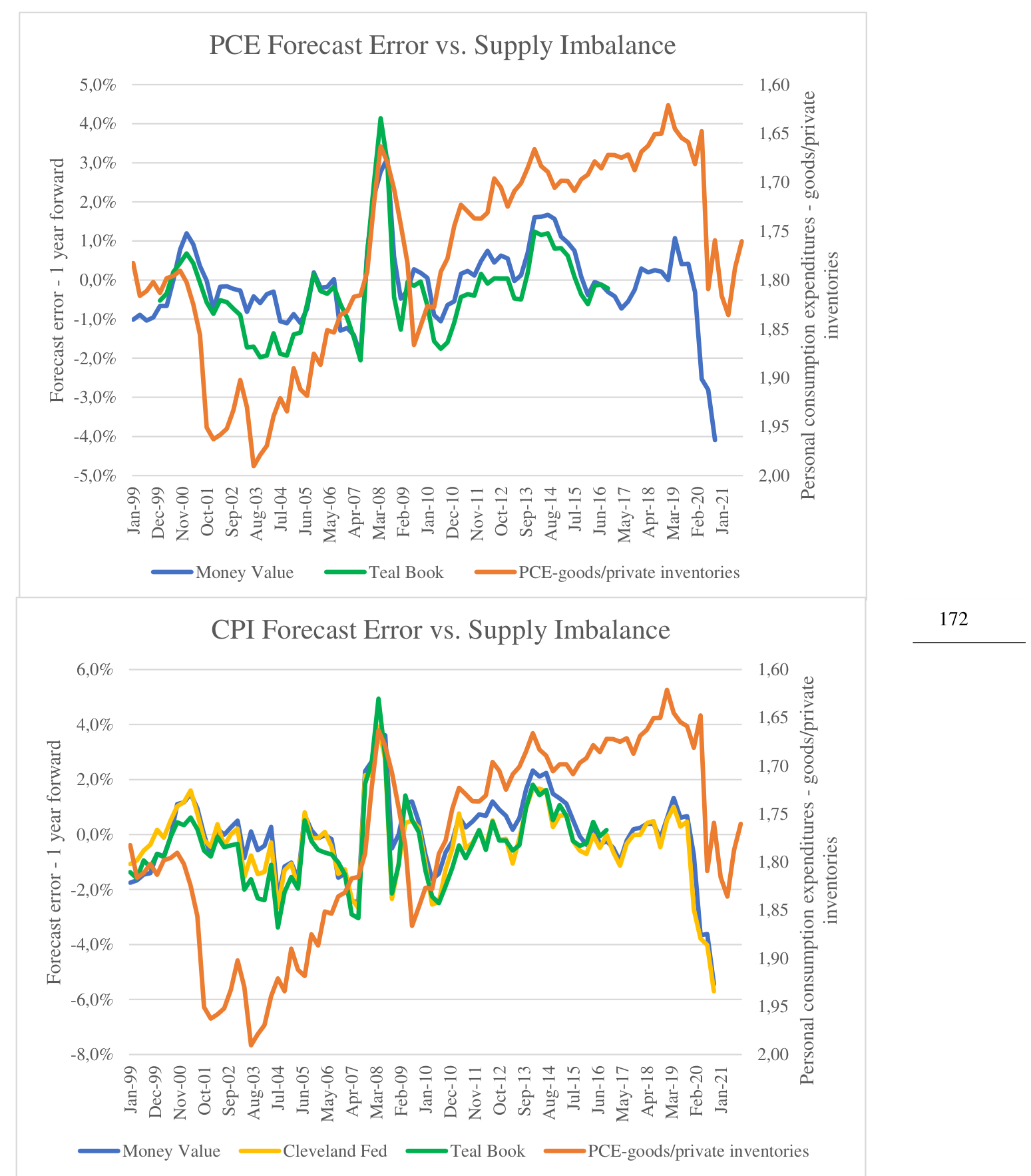
Noteworthy is how the different forecast methodologies produce similar forecast errors. Demand/supply imbalance contributes to the errors. Tables 13 and 14 contain regression statistics for this relationship.
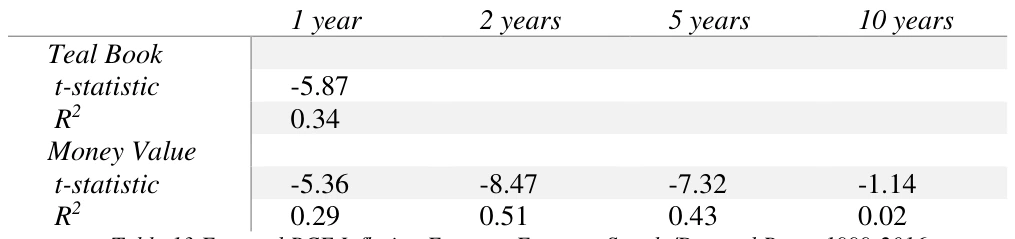

In the short to medium term there is a very significant relationship between the demand/supply proxy and forecast errors, but it fades almost completely by 10 years. The Cleveland Fed market-derived expectations measure is less affected by the imbalances than the monetary Money Value model.
6.2.2. Money Value and Real Economic Growth
The earlier Money Value analysis focused on inflation. Could a similar diminishing effect of monetary stimulus apply to real growth?
Figure 11 carries over the Money Value price effect to aggregate demand, assuming initial price stickiness. In Figure 4, a percentage increase in money, %dM, has a much larger effect on the unit value of money in the elastic state, moving it from m1a to m1b, a much greater change than in the inelastic region where the unit value moves from m2a to m2b.
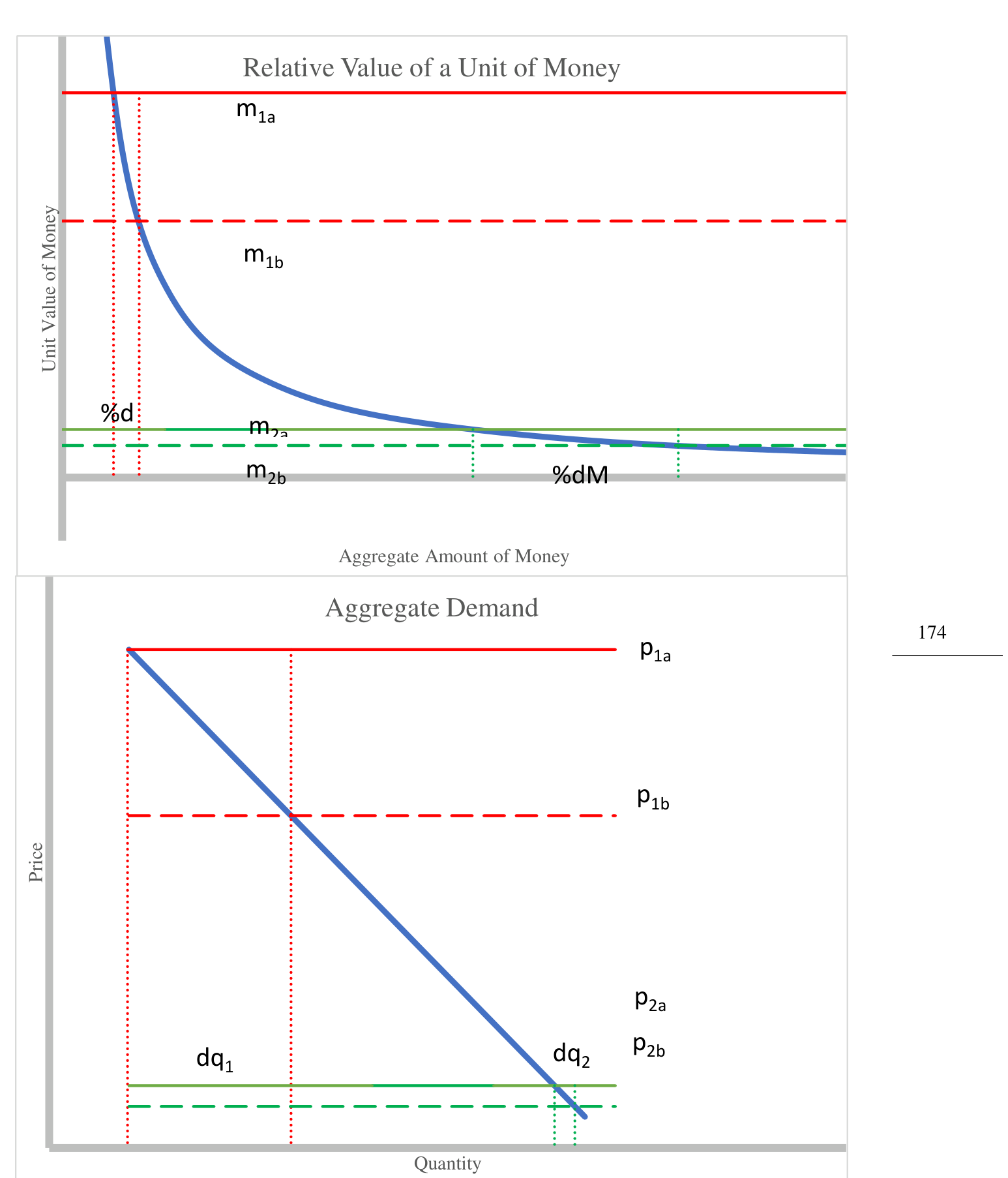
Depending upon the elasticity of aggregate demand, the money value effect will have different effects. Constantly elastic aggregate demand may offset the Money Value elasticity, while, as shown in Figure 11b, varying elasticity of price effects, p1a to p1b and p2a to p2b respectively, produce dramatically different quantity effects, dq1 and dq2.
To evaluate the potential monetary effect upon real GDP, Table 15 compares a lag of M2 using the Money Value formula while Table 16 makes the same comparison with straight percentage growth of M2


While far from its statistical relationship with inflation, the Money Value formula provides a superior explanation of a monetary effect on real growth with higher statistical fit, lower standard errors, and intercepts corresponding to actual real growth levels.
A similar comparison is made for nominal GDP growth between monetary effects calculated from the Money Value formula in Table 17 and straight percentage figures in Table 18.


Again, for nominal GDP, the Money Value formula provides a significantly superior statistical fit.
7. Financial Stability Risks
The preceding analysis highlights a couple of major potential risks for monetary policy.
7.1. Inflation Target Surprise and Asset Bubble Risks
The Money Value formula suggests monetary stimulus has a geometrically declining effect upon inflation, real growth, and thus upon incomes. Where does excess credit generated above and beyond this diminished income growth go? Assets. In earlier Figure 4a comparing monetary value with quantity, 1996 is around the time when the inelasticity of monetary stimulus began to prevail. Figure 12 depicts the indexed path for money, asset prices, and income since that time.
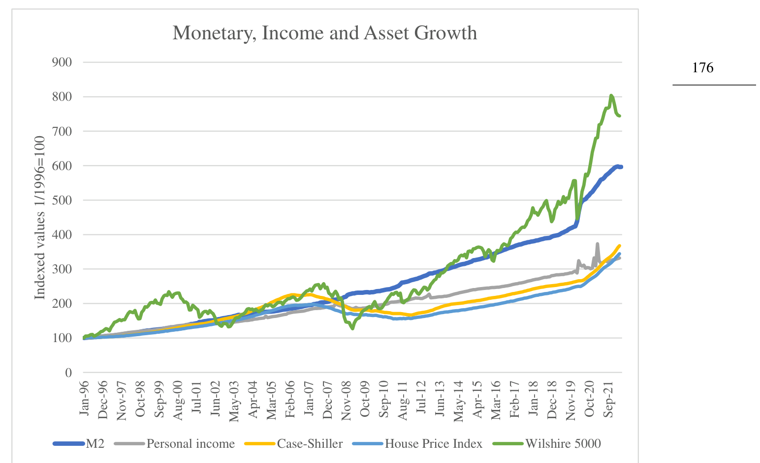
Monetary growth and stock prices far exceed the growth in personal income during the post-1996 period. Housing prices barely outperform income following a big hit in the Great Financial Crisis aftermath after housing had outperformed income for years. Figure 13 provides a similar illustration of the pre-1996 period.
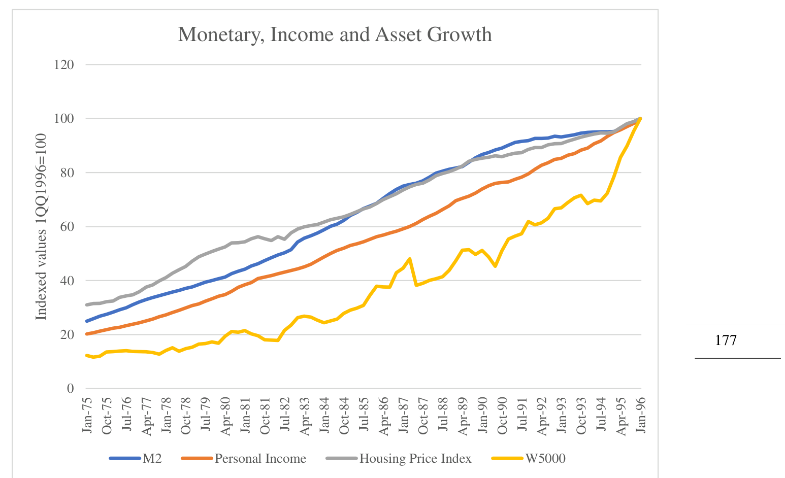
In the monetary elasticity regime prior to 1996, incomes outgrew money and home prices. Stock prices from the depressed mid-1970 stock market outgrew personal income, but, from the beginning of the 1970’s, stocks and incomes grew evenly.
In the recent inelastic period, home price increases above income growth already produced one major crisis. Figure 14 displays home prices relative to disposable personal income.

The level of home prices to disposable personal income is at virtually the same level as preceded the Great Financial Crisis. Depending upon the home price measure this level may have been exceeded once before in the 1970’s when double digit inflation boosted home prices and resulted in very negative real after-tax mortgage rates. Even the current housing market doesn’t face those conditions.
Asset bubble risks from over stimulus will be compounded in the future if, as the Money Value model predicts, inflation in advanced economies resumes its long downtrend. Figure 15 depicts the path of Natural Inflation in the three largest advanced economic areas.

Natural Inflation, an important determinant of overall inflation, has been steadily declining in advanced economies for 50 years. Components of the natural inflation rate, natural interest that reflects economic growth and population growth have been in decline throughout this period and no end is in sight. Monetary inflation is diminishing geometrically in the Money Value model, and fiscal inflation can’t continue indefinitely from constantly climbing deficits.
Asset bubble risk is compounded when central bank inflation targets are higher than an economy’s naturally occurring inflation rate evident in its actual performance.
7.2. The Fiscal Inflation Surprise and Policy Mismatch Risks
Earlier sections on monetary and cyclical inflation factors describe entirely different characteristics, suggesting monetary policy may not be an ideal tool for curing fiscal inflation.
The pandemic era inflation does not appear to have monetary origins. Figure 16 compares actual inflation to regression estimates for the Money Value model.
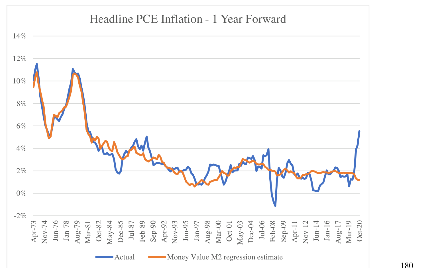
The regression closely tracks actual data, even though the volatile 1970’s. Exceptions are the Great Financial Crisis and the pandemic. This paper’s second section described how fiscal and trade balances likely produced the pandemic era error.
The fiscal effect identified in that section was dramatically different than what was previously identified as the monetary effect upon inflation. In the Money Value framework, changes in money’s value occur over more than a decade. Fiscal effects are immediate, largely within a year. Figure 17 compares the statistical significance of lagged monetary and fiscal effects upon inflation.

The effects on short-term inflation of monetary stimulus seem to linger for more than 18 years. Fiscal stimulus effects decline to insignificance after two years then reverse reflecting cyclical correlation.
The contrast between monetary and fiscally induced inflation is evident in comparing the Great Inflation, with monetary origins evident in Figure 16, to the fiscal inflation arising from the pandemic. Figure 18 compares each inflation from shortly before inflation rose past 2% to its peak level.
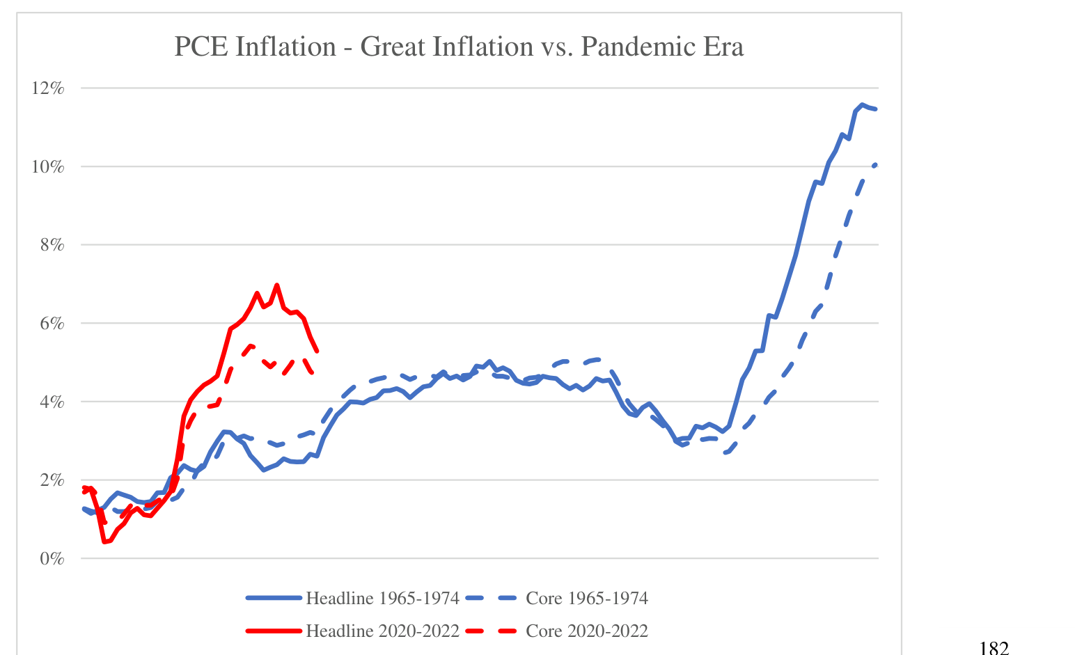
As recently as February 2021 in the pandemic era, annual PCE inflation was under 2%. Its peak was 6.6% in March 2022. The fiscal effect was immediate. In contrast, preceding the monetary Great Inflation, inflation was last below 2% in January 1965 and did not reach 6.6% until October 1973.
The very different responses of inflation to fiscal and monetary stimulus suggest using monetary policy to offset fiscal policy will produce a mismatched response. Of course, optimal fiscal adjustments can be difficult politically, complicating the policy response. The significantly reduced response of inflation to monetary stimulus that characterized the pre-pandemic era will apply to bringing inflation down as well as the previous attempt to bring it up. Fortunately, fiscal policy tends to swing automatically with the economy and may ease the otherwise difficult policy adjustment.
8. Conclusion
The paper presents an entirely new framework for understanding the causes of inflation, which has three fundamental components.
The first major inflation determinant is the Natural Rate of Inflation, an underlying base level of inflation related to an economy’s dynamism as reflected in its population growth and its natural rate of interest, which, in turn, reflects economic growth. Natural Inflation varies only gradually, with little effect from monetary policy or business cycles.
The second major inflation factor is the value of money, a function of monetary aggregates within a model to determine the money’s relative unit value. The formula explains virtually all long-term variability of inflation (5+ years) and is characterized by geometrically diminishing effects of monetary stimulus upon inflation, or inflation inelasticity. This geometric decline also is evident in diminishing effects of monetary stimulus upon real growth.
The third inflation component is cyclical influences. Fiscal balance is the policy lever in this category, and external balance and demand shifts also have impact. Cyclical factors are difficult to ascertain directly against inflation data, but, analysed within the Money Value model framework, their effect is evident. Cyclical factors account for much of the short-term variability of inflation and typically produce effects within a year that don’t last much longer than another year. During the QE era, fiscal deficits stimulating consumption and trade deficits enhancing supply were exceptionally significant in determining inflation variability, perhaps because other policy tools or influences remained stuck in one position.
Combined, these factors account for the major monetary surprises in recent history. The dampened responsiveness of inflation to monetary stimulus since the 1990’s accompanies an increased prevalence of financial bubbles triggering business cycles. This was the period in the U.S. when the response of inflation to monetary stimulus evolved from elastic to inelastic. With incomes falling behind growth in money, credit, and asset prices, occasional readjustments became the norm. Other advanced economies experienced similar phenomena around this time.
At the height of the Great Financial Crisis, inflation was more resilient than expected, albeit at a low level. This reflected the Natural Inflation Rate, which set a floor on inflation and was unresponsive to monetary or business cycle disturbances.
Finally, and most recently, the pandemic burst of inflation and forecasting shortfalls are both largely explained by cyclical factors from the twin deficits, especially with the unprecedented magnitude of U.S. fiscal deficits.
It will be evident to readers that this paper’s framework stands in contrast to conventional inflation theory. Among the contrarian implications of this framework are:
- Fiscal and monetary policy have entirely different effects upon inflation and aggregate demand. Fiscal policy affects consumption directly and takes about a year to filter through to prices, with effects lingering for about another year (although difficult to evaluate with unprecedented U.S. deficits.) Monetary policy has limited immediate impact in current inelastic economies, and its price effect
filters through over years in a dialectic process between the unit value of a currency and values of goods and services. 2) Inflation is likely to resume its sub-2% target path in advanced economies. Natural Inflation in advanced economies has been in and will continue to be in decline. Inflation determinants, population growth and natural interest (along with economic growth), have been declining now for decades. At the same time inelastic inflation prevails in major advanced economies, rendering monetary stimulus ineffective at spurring inflation. Yawning projected government deficits in the U.S. may exert upward pressure on inflation but are likely to be at least somewhat offset by trade deficits, and no projection compares with the extraordinary pandemic borrowing of 20% of GDP. 3) Central banks are neither responsible for nor do they possess solutions to the inflation surprises of recent years. Inflation inelasticity suggests an inability to fine tune inflation rates beyond what the Natural Inflation and cyclical factors dictate. In the short-term, central banks can influence foreign exchange rates with a consequent effect on short-term inflation, but this reverses with foreign exchange swings.
A. APPENDIX – THE MONEY VALUE MODEL
This appendix provides further information on the specification and results of the Money Value monetary inflation model utilized in the paper’s main body.
There are a variety of monetary measures that could be tested against inflation, and, for testing purposes, specificity must be given to the “long and variable lags” that are believed to link money and inflation. Figure A-1 measures the statistical significance to one year forward headline PCE inflation of various monetary aggregates for single lagged years back fifteen years from estimation.
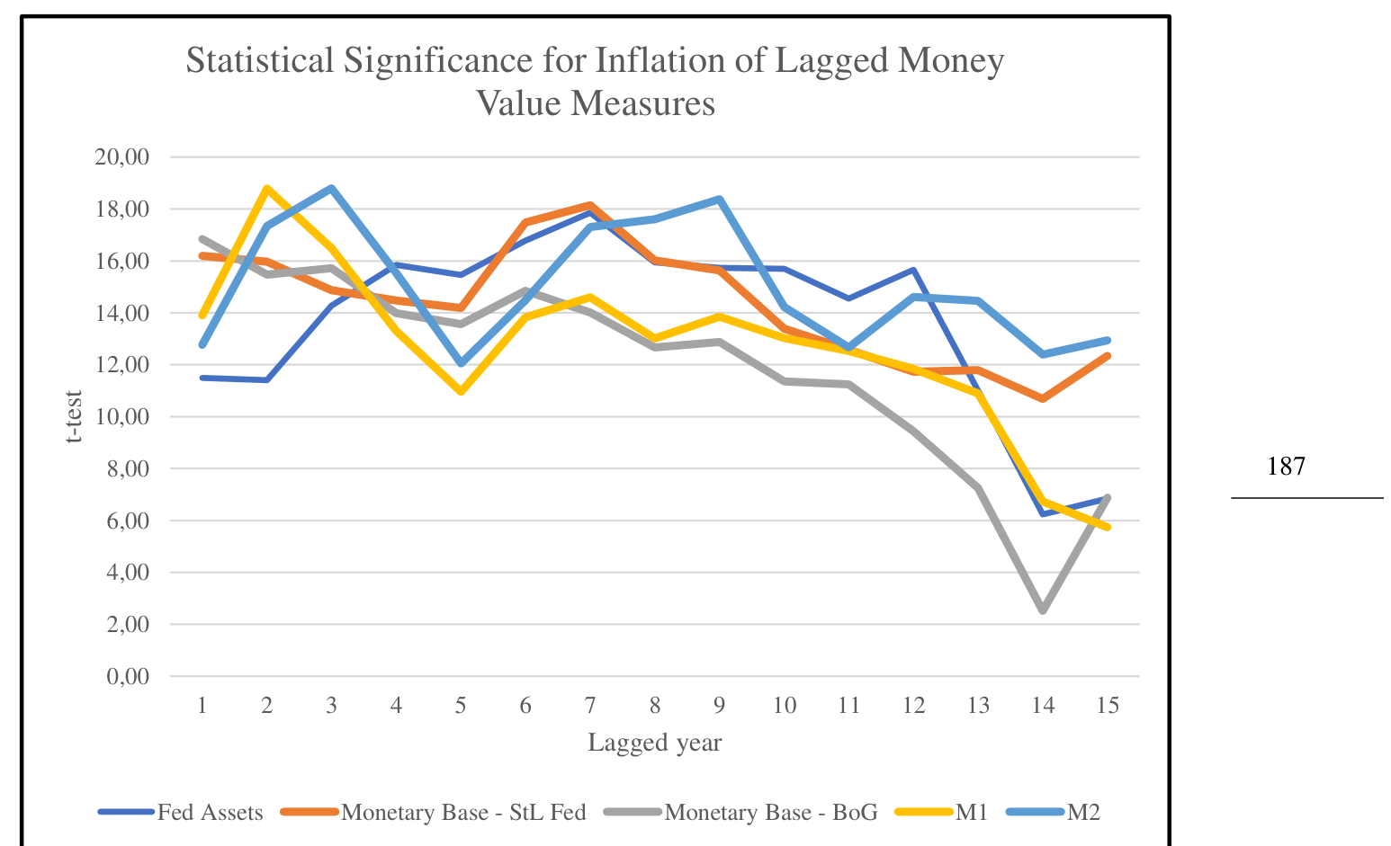
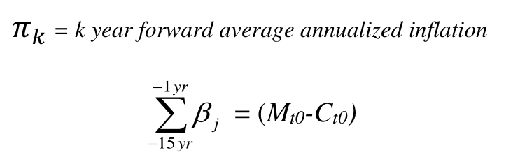
Up to at least fifteen years, all the various measures exhibit a significant relationship with one year forward inflation. The regression equation used throughout this paper thus becomes:

where
In Figure A-2, Equation A-1 is regressed with a variety of monetary aggregates in a 15 year lag:
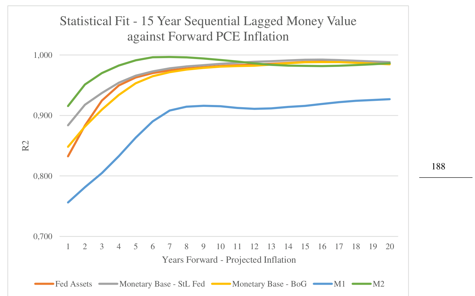
Again, all aggregates were found to explain a very high amount of the variation in forward inflation rates, especially over longer time horizons beyond 5 years where 95-99% of the variation of inflation rates is explained by the Money Value Formula. The various aggregates are highly correlated with each other, so, for the most part, results are comparable, but M1, which has had well-known shifts in usage, is an outlier with lower statistical fit at all horizons. Measures used include credit statistics such as Fed assets, as well as traditional monetary aggregates.
The strong connection between lagged aggregates and inflation is attributable to the Money Value Formula. Figure A-3 compares regression results from the Formula with the exact same regression specification using straight percentage growth associated with the Quantity Theory.

The Money Value Formula increased the explanatory power of lagged M2 by 50-80% over straight percentage growth associated with the Quantity Theory.
A.1. U.S. Regression Results
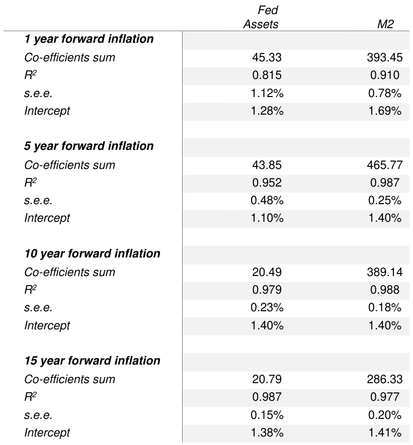
Equation A-1 is tested empirically against post World War II data in the U.S., with ordinary least squares regressions. Table A-1 contains data for headline PCE inflation while Table A-2 contains data for core PCE inflation. Both the broader M2 measure and the narrow measure of Federal Reserve assets were used as aggregates.
1 For multivariable sequential lagged regressions, the high degree of multicollinearity between lagged data renders coefficients and thus t-statistics not meaningful, although equations may provide valid forecasts.
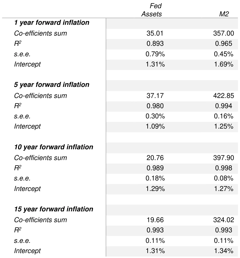
Both aggregates provide significant explanatory power for future inflation, especially as horizons lengthen beyond five years with estimate standard errors also dropping considerably. With the Money Value Formula, long-term inflation regressions explain more variability than short-term forecasts.
In the paper’s Equations 4 and 5, the constant Mt0 was not specified but should be similar to the aggregate’s initial value or minimum. In 1959, the beginning of the time period for the lagged regressions in Table A-1, the initial value for Fed Assets was $52.7 billion, currency was $31.2 billion, and M2 was $289.2 billion, so co-efficients are statistically comparable to initial values of $21.5 billion for Fed assets and $258.0 billion for M2, as would be expected from the original theoretical formulation.
All regressions have an intercept between 1.00-1.70%, suggesting this is a residual or base level of price increases that is not affected by U.S. monetary policy.
Estimates from these regressions closely match actual results as depicted for 10 year forward inflation in Figure A-4.

A.2. International Regression Results
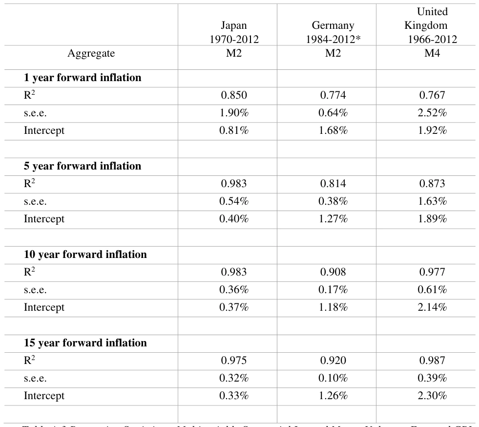
Table A-3 contains historical regression analysis for these advanced economies. The period studied for each economy was the longest period possible with data available in the U.S. for monetary aggregates and inflation figures. For Japan and Germany, M2 provided the longest accessible history, while, for the UK, M4 provided the deepest history. Of course, Germany experienced a transition from its own Deutsche Mark to the Euro. Data for the two currencies was combined to realize longer history, although there likely is a loss of precision. Through 1998, domestic German money supply data was used, while, afterwards, money supply for the entire Euro Area was used. As with the U.S. data, Equation 14 was the model for regression evaluation.
Accessible table text
| — | Japan 1970-2012 | Germany 1984-2012* | United Kingdom 1966-2012 |
|---|---|---|---|
| Aggregate | M2 | M2 | M4 |
| 1 year forward inflation | — | — | — |
| R2 | 0.850 | 0.774 | 0.767 |
| s.e.e. | 1.90% | 0.64% | 2.52% |
| Intercept | 0.81% | 1.68% | 1.92% |
| — | — | — | — |
| 5 year forward inflation | — | — | — |
| R2 | 0.983 | 0.814 | 0.873 |
| s.e.e. | 0.54% | 0.38% | 1.63% |
| Intercept | 0.40% | 1.27% | 1.89% |
| — | — | — | — |
| 10 year forward inflation | — | — | — |
| R2 | 0.983 | 0.908 | 0.977 |
| s.e.e. | 0.36% | 0.17% | 0.61% |
| Intercept | 0.37% | 1.18% | 2.14% |
| — | — | — | — |
| 15 year forward inflation | — | — | — |
| R2 | 0.975 | 0.920 | 0.987 |
| s.e.e. | 0.32% | 0.10% | 0.39% |
| Intercept | 0.33% | 1.26% | 2.30% |
| — | — | — | — |
All three major economies had strong statistical fits between the Money Value model and forward inflation. Germany provided a lesser, although still significant, fit, likely due to the combination of currencies necessary for the analysis. Once again, the fit improved and error declined at longer horizons. Of note was the low regression constant for Japan’s CPI of 0.3-0,4%, suggesting a very low level of base inflation from non-monetary causes. Germany’s regression intercept base inflation level also was significantly below the European Central Bank’s 2% inflation objective.
A.3. Forecasting Inflation – International
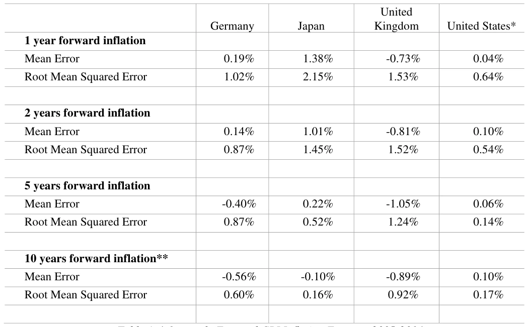
Out-of-sample forecast evaluation also was done for the major economies with a comparison to the U.S. for years 2005-2014 in Table A-4.
Accessible table text
| — | Germany | Japan | United Kingdom | United States* |
|---|---|---|---|---|
| 1 year forward inflation | — | — | — | — |
| Mean Error | 0.19% | 1.38% | -0.73% | 0.04% |
| Root Mean Squared Error | 1.02% | 2.15% | 1.53% | 0.64% |
| — | — | — | — | — |
| 2 years forward inflation | — | — | — | — |
| Mean Error | 0.14% | 1.01% | -0.81% | 0.10% |
| Root Mean Squared Error | 0.87% | 1.45% | 1.52% | 0.54% |
| — | — | — | — | — |
| 5 years forward inflation | — | — | — | — |
| Mean Error | -0.40% | 0.22% | -1.05% | 0.06% |
| Root Mean Squared Error | 0.87% | 0.52% | 1.24% | 0.14% |
| — | — | — | — | — |
| 10 years forward inflation** | — | — | — | — |
| Mean Error | -0.56% | -0.10% | -0.89% | 0.10% |
| Root Mean Squared Error | 0.60% | 0.16% | 0.92% | 0.17% |
| — | — | — | — | — |
*U.S. forecasts based upon M2 aggregate **10-year forecasts evaluated through 2009
Errors were significantly higher for Germany, Japan, and the UK than for comparable U.S. forecasts, which has had longer and more comprehensive development with the Money Value model. Nevertheless, at longer horizons, errors were generally smaller for Germany and Japan than for comparable U.S. forecasts in the Survey of Professional Forecasters. Additional data and refinement may present opportunities for improving international forecasting results.
B. APPENDIX – THE NATURAL RATE OF INTEREST
Knut Wicksell (1936) famously described his concept of the natural rate of interest as:
...a certain rate of interest on loans which is neutral in respect to commodity prices and tends neither to raise nor to lower them.
Since Woodford (2003) incorporated the natural interest rate concept into New Keynesian models, the subject has received renewed focus whether in comprehensive structural models such as Andrés et al (2008), Barsky et al (2014), and Cúrdia et al (2015) or in reduced form specifications such as Laubach and Williams (2002, 2016) and Holston et al (2017). All the New Keynesian variants determine the natural rate with a Phillips curve and IS equation, so it is a function of economic agents’ time preference between consumption and savings. These relationships can be problematic. Blanchard (2016), while defending the Phillips curve, stated, “The relationship has never been very tight.” Hamilton et al (2015) state, “Unfortunately, a huge literature has documented that [the IS equation] does not work well empirically,” citing Kocherlakota (1996) and Mehra and Prescott (2003). Hamilton et al go on to test autoregressive functions of interest rates and economic variables. Lubik and Matthes (2015) and Johanssen and Mertens (2018) also perform autoregressive analyses. All find interesting and relevant conclusions on the path of natural interest rates, but there seems no disputing Hamilton et al saying, “A key conclusion of our analysis is that the uncertainty around the equilibrium interest rate ...is very considerable,” as is naturally the case for an unobservable variable.
Ironically, the impressive analytical firepower applied in these studies has been directed at the intersection of time preference and what Wicksell would refer to as the “money rate of interest,” whereas Wicksell was focused on the intersection of this “money rate” and what he called “the natural rate of interest on capital.”
...the rate of interest which would be determined by supply and demand if no use were made of money and all lending were effected in the form of real capital goods.
For Wicksell, the natural rate:
...depends on the efficiency of production, on the available amount of fixed and liquid capital, on the supply of labour and land, in short on all the thousand and one things which determine the current economic position of a community; and with them it constantly fluctuates.
To compare “money rates” with real capital returns, short-term riskless financial yields will be compared with the productivity of capital, specifically the capital factor share of incremental growth from capital investment.
B.1. Incremental Growth from Capital Investment
To determine the incremental growth from capital, a simple model for the relationship between capital investment and growth is developed, which will then be combined with applicable capital productivity as the capital factor share producing a proxy for the natural rate. A generalized growth model is represented as:
,...),, ( 2 1 t t t t X X K f Y = where
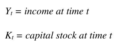

Accordingly, income growth comes from the productivity of capital multiplied by capital investment:

where

Participants in the economy wish to maximize growth, which occurs when the first derivative of growth Equation B-1 equals zero:
0 = + = dk dp k p dk dy k k
Therefore, at any given point in time, there are declining returns to investment as capital productivity declines with greater investment:

While declining at any given instant, capital productivity need not decline over time, as other production factors such as technology or labour growth can increase capital productivity to offset diminishing returns.
The other side of investment is the decision to save for investment rather than consume. The IS equation, found troublesome above, is replaced with a direct comparison of consumption and capital’s product. Consumption is:

where
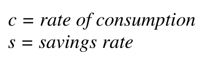
so

For a simplified closed economy:

Since the income produced by investment can be used for consumption, participants in an economy will continue to invest as long as marginal investment productivity is greater than the decline in consumption from increased savings. Indifference occurs at the equality from Equations B-2 and B-3:
1 − = = − = ds dc k p dk dp k k
To this point, participants gain more from marginal investment than from consumption. At indifference:

Combining equations B-1 and B-4 produces:

While new investment adds to growth, depreciation of existing investment detracts from it, and capital productivity must be higher to offset depreciation. If capital productivity lost from depreciation is comparable to that of new investment, Equation B-5 is written as:

where

Equation B-6 produces an estimate analogous to steady state potential growth. Investment ratio changes affect the capital product, but the changes themselves are part of income and must be incorporated to capture cyclical effects.

where
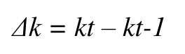
Accordingly, this Investment-Growth Model represents growth as the product of net investment and the sum of investment and depreciation with an additional term for investment rate changes. As opposed to the New Keynesian bottom-up use of agents, this model’s marginal conditions are applied top-down directly to the macro economy. The investment-consumption trade-off is made on the basis that investment will not be made beyond the point where incremental production is worth less than forgone consumption.
B.1.1. Empirical Analysis
Equation B-7 utilizes the sum of investment and depreciation (k+d) as equivalent to capital productivity. Back in Equation B-1, the output/capital ratio (Y/K) was utilized. The Bureau of Labor Statistics and the San Francisco Federal Reserve Bank also produce capital productivity measures, all of which are similar in magnitude, as illustrated in Table B-1:

Plugging these capital productivity factors into Equation B-7 results in the Table B-2 error statistics when compared with actual annual real GDP growth in the U.S.:

Accessible table text
| — | — | — | k+d | — | — | — | BLS | SF Fed alpha |
|---|---|---|---|---|---|---|---|---|
| — | — | — | — | — | 𝑌 𝐾 | — | — | — |
| — | Mean Error | — | -0.22% | -0.21% | -0.21% | — | -0.37% | -0.51% |
| — | RMSE | — | 1.19% 1.23% 1.23% 1.29% | — | — | — | — | — |
The Investment-Growth model produces estimates based on contemporaneous data and not forecasts, but it is instructive, given the model’s sparseness, to compare its estimates with GDP growth forecasts with RMSE’s that typically run from 1.00-1.50% [Stark 2018].
Figure B-1 compares actual real U.S. GDP growth with estimates from the model using the various capital productivity factors.
2 Economic statistics are from FRED, including Penn World Tables for output and capital stock. BLS and San Francisco Fed data are from source.

The Investment-Growth model also can be evaluated against data from a panel of OECD economies. Table B-3 contains regressions for average actuals and estimates for countries and periods shown in Table B-4:
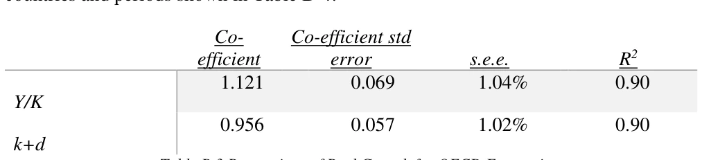
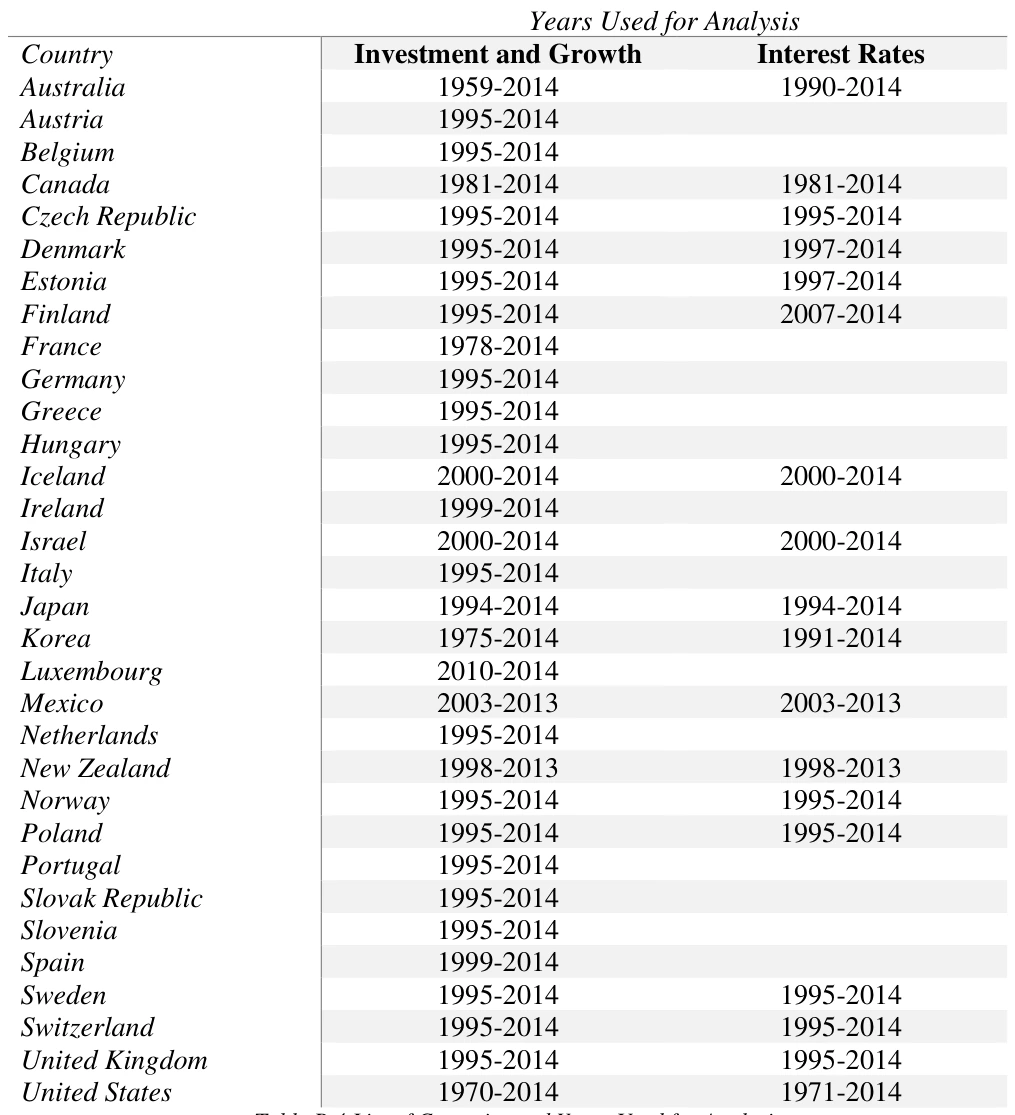
Accessible table text
| — | — | — | — | Years Used for Analysis | — | — | — | — |
|---|---|---|---|---|---|---|---|---|
| — | Country | — | — | Investment and Growth | — | — | Interest Rates | — |
| — | Australia | — | 1959-2014 1990-2014 | — | — | — | — | — |
| — | Austria | — | — | 1995-2014 | — | — | — | — |
| — | Belgium | — | 1995-2014 | — | — | — | — | — |
| — | Canada | — | — | 1981-2014 | — | — | 1981-2014 | — |
| — | Czech Republic | — | 1995-2014 1995-2014 | — | — | — | — | — |
| — | Denmark | — | — | 1995-2014 | — | — | 1997-2014 | — |
| — | Estonia | — | 1995-2014 1997-2014 | — | — | — | — | — |
| — | Finland | — | — | 1995-2014 | — | — | 2007-2014 | — |
| — | France | — | 1978-2014 | — | — | — | — | — |
| — | Germany | — | — | 1995-2014 | — | — | — | — |
| — | Greece | — | 1995-2014 | — | — | — | — | — |
| — | Hungary | — | — | 1995-2014 | — | — | — | — |
| — | Iceland | — | 2000-2014 2000-2014 | — | — | — | — | — |
| — | Ireland | — | — | 1999-2014 | — | — | — | — |
| — | Israel | — | 2000-2014 2000-2014 | — | — | — | — | — |
| — | Italy | — | — | 1995-2014 | — | — | — | — |
| — | Japan | — | 1994-2014 1994-2014 | — | — | — | — | — |
| — | Korea | — | — | 1975-2014 | — | — | 1991-2014 | — |
| — | Luxembourg | — | 2010-2014 | — | — | — | — | — |
| — | Mexico | — | — | 2003-2013 | — | — | 2003-2013 | — |
| — | Netherlands | — | 1995-2014 | — | — | — | — | — |
| — | New Zealand | — | — | 1998-2013 | — | — | 1998-2013 | — |
| — | Norway | — | 1995-2014 1995-2014 | — | — | — | — | — |
| — | Poland | — | — | 1995-2014 | — | — | 1995-2014 | — |
| — | Portugal | — | 1995-2014 | — | — | — | — | — |
| — | Slovak Republic | — | — | 1995-2014 | — | — | — | — |
| — | Slovenia | — | 1995-2014 | — | — | — | — | — |
| — | Spain | — | — | 1999-2014 | — | — | — | — |
| — | Sweden | — | 1995-2014 1995-2014 | — | — | — | — | — |
| — | Switzerland | — | — | 1995-2014 | — | — | 1995-2014 | — |
| — | United Kingdom | — | 1995-2014 1995-2014 | — | — | — | — | — |
| — | United States | — | — | 1970-2014 | — | — | 1971-2014 | — |
B.2. Natural Rate Of Interest
The natural rate of interest then results from the incremental potential growth from capital, derived above, multiplied by the capital factor share, which equals the productivity of capital.


B.2.1. Empirical Analysis
The various capital productivity measures in Equation B-8 are compared in Table B-5 with well-known Laubach-Williams estimates and with real T-bill rates for the U.S. calculated from nominal yields less two year lagged core PCE inflation (or PCE when core figures are unavailable).3

Accessible table text
| — | Current Quarter | — | — | Mean Error | — | — | RMSE | — |
|---|---|---|---|---|---|---|---|---|
| — | k+d | — | -0.47% | -0.47% | — | 1.98% | 1.98% | — |
| — | SF Fed alpha | — | -0.67% 2.14% | — | — | — | — | — |
| — | LW 1 -sided | — | 1.56% | — | — | 2.59% | — | — |
| — | LW 2-sided | — | 1.22% 2.22% | — | — | — | — | — |
The Model has lower errors, but none of the estimates are consistent with observed market T-bill rates, which have a great deal more volatility as indicated in Figure B-2.
3 Williams (2015) found lagged inflation approximated inflation expectations. 4 Output/capital stock and BLS measures of capital productivity were not available on a quarterly basis and are excluded from this analysis.

Figure B-2 transforms the real yields from Figure B-3 into nominal yields using three year lagged CPI inflation.
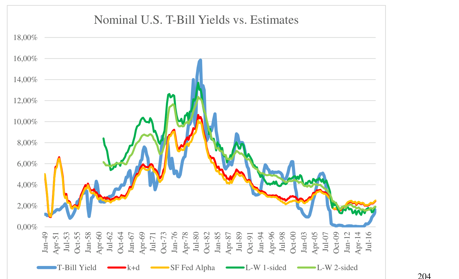
Nominal natural rate estimates are generally comparable to market rates, but with significantly less volatility. One of the larger variances is during the Quantitative Easing era. As will be explored in a later section, central bank balance sheet activity has a major effect upon short-term market rates and is the logical cause of the discrepancy.
The Investment-Growth model formulas for Natural Interest are checked against OECD data with regressions in Table B-6. Sample countries are specified in Table B-4 and exclude Euro area economies with the common currency’s effect upon rates. Nominal market interest rates are transformed to real rates by deducting trailing four year average GDP deflator inflation.

Accessible table text
| Co- Co-eff efficient std e | — | icient rror s.e.e. R2 | — |
|---|---|---|---|
| — | 0.954 0 k+d | .023 2.68% 0.82 | — |
| — | Y/K 1.014 0 | .024 2.68% 0.82 | — |
The pooled cross section and time series sample for Table B-6 includes a variety of economies from Slovenia to the United States and makes no adjustment for central bank policies or other influences upon interest rates but is broadly consistent with the Model as illustrated in Figure B-4.

C. APPENDIX – FORWARD INFLATION FORECASTS
In addition to models, surveys and market rate data are used to forecast future inflation. To evaluate long-term inflation forecasts, long time series are needed. Among consumer surveys, the University of Michigan Surveys of Consumers provide a suitably long track record. For professional surveys, the Philadelphia Federal Reserve’s Livingston Survey also has a long track record compared with their Survey of Professional Forecasters. The similarly long Blue Chip Survey is proprietary and unavailable for this research. Since the innovation of Treasury Inflation Protected Securities (TIPS), simple breakevens, the difference between real and nominal bonds, have been available as an inflation indicator. A more sophisticated measure of financial market inflation expectations is provided by the Cleveland Fed (Haubrich et al 2012), and the Board of Governors staff also produces a sophisticated expectations measure, the Index of Common Inflation Expectations (CIE) (Ahn and Fulton 2020). Along with the Money Value model, these inflation expectations and forecasts include examples of most approaches to estimating future inflation.
C.1. Long-Term Forecasts
University of Michigan, Livingston, and Cleveland Fed measures begin around 1980, but the Money Value model with its long leads and lags (15 years back and as many as 10 years forward) doesn’t become stable until later, so, for data available by then, the forecast evaluation begins in 1990. The CIE series begins in 1999, and TIPS breakeven data becomes available in 2003, so additional evaluations will begin in those years. Forecasts will be examined for their mean error and root mean squared error.
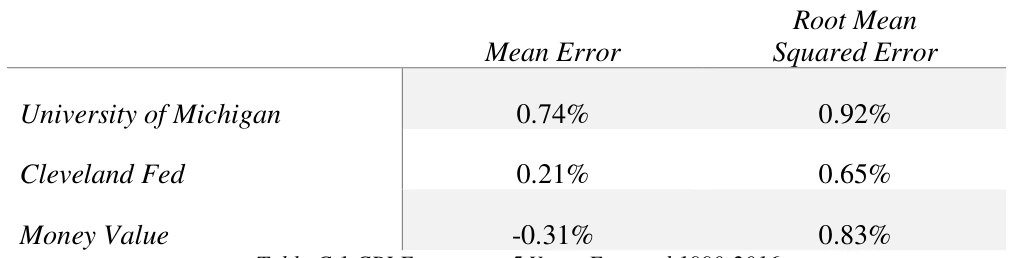
Figure C-1 displays actuals versus forecasts of 5 year forward CPI inflation, while Tables C-1 and C-2 contain error statistics for the forecasts. Table C-3 contains correlations and variability of the forecasts.

Accessible table text
| Mea | — | Root Mean n Error Squared Error | — |
|---|---|---|---|
| — | University of Michigan 0 | .74% 0.92% | — |
| — | Cleveland Fed 0 | .21% 0.65% | — |
| — | Money Value -0 | .31% 0.83% | — |

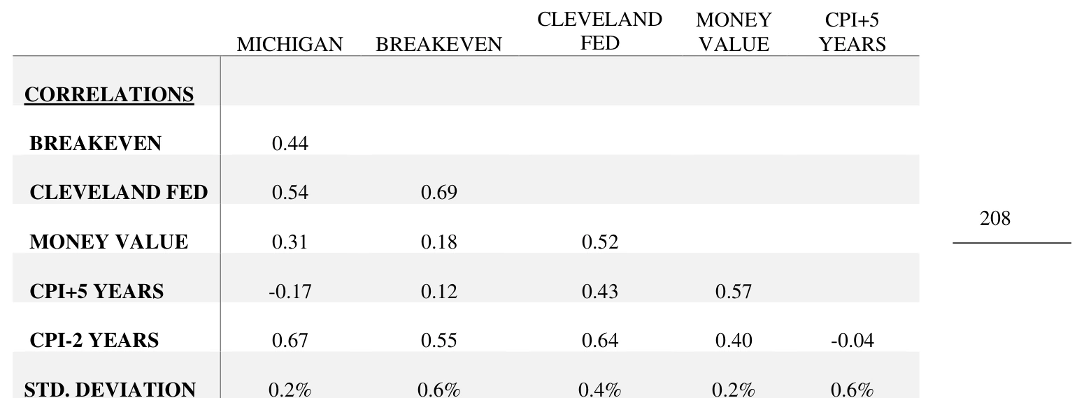
The Michigan Survey does not ask for exactly what is being evaluated in this analysis. Respondents are asked to estimate inflation in 5 years and not over 5 years, which may explain some of its lesser performance. Of course, a representative consumer sample consists of about half of respondents who are unable to do financial computations, so its accuracy may be questioned. It has a consistent overestimate that may possibly be related to the quality adjustments made in official inflation measures. TIPS breakevens, the Cleveland Fed, and Money Value model are reasonably comparable and highly correlated, interesting with such different approaches. All the forecast methods are highly correlated with historical inflation.
Figure C-2 displays actuals versus forecasts of 10 year forward CPI inflation, while Tables C-4 and C-5 contain error statistics for the forecasts, with Table C-6 containing correlations and variability for the forecasts.

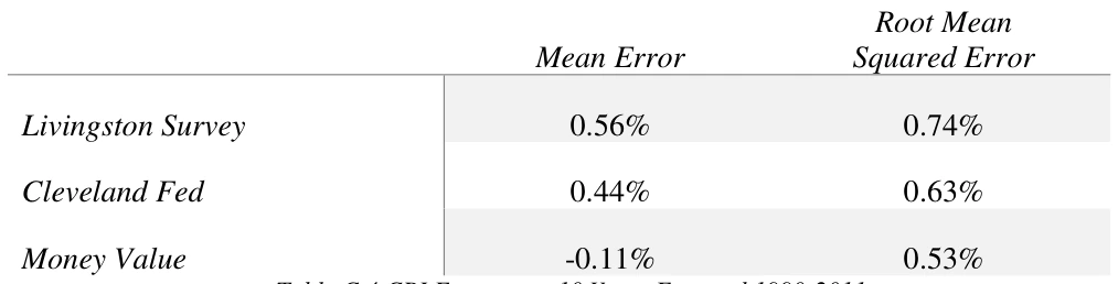
Accessible table text
| M | — | Root Mean ean Error Squared Error | — |
|---|---|---|---|
| — | Livingston Survey | 0.56% 0.74% | — |
| — | Cleveland Fed | 0.44% 0.63% | — |
| — | Money Value | -0.11% 0.53% | — |
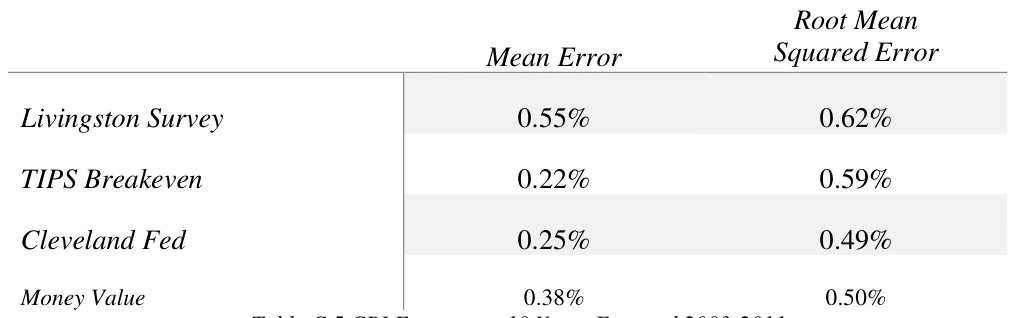
Accessible table text
| — | — | Mean Error | — | — | Root Mean | — |
|---|---|---|---|---|---|---|
| — | — | — | — | — | Squared Error | — |
| — | Livingston Survey | 0.55% | — | — | 0.62% | — |
| — | TIPS Breakeven | 0.22% 0.59% | — | — | — | — |
| — | Cleveland Fed | 0.25% | — | — | 0.49% | — |
| — | Money Value | 0.38% 0.50% | — | — | — | — |
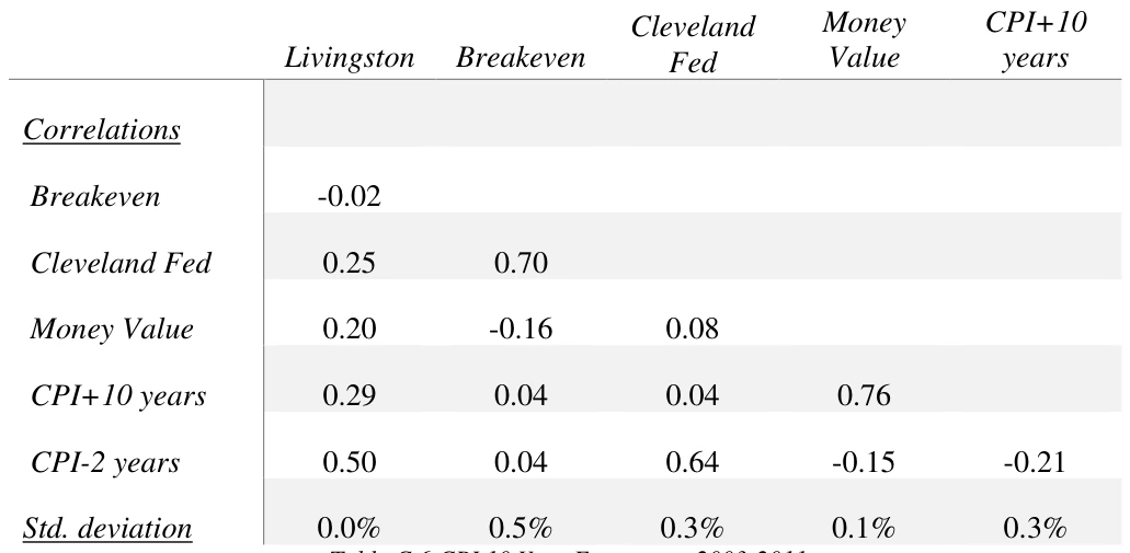
Again, the forecasts are reasonably close, although there appears some benefit to the more rigorous methodology of the Cleveland Fed and Money Value forecasts. The 10 year forecasts are at least as accurate as the preceding 5 year forecasts. Unusually, the breakeven measures are more volatile than the objective inflation measure and are highly correlated with the Cleveland Fed measured, both being market-derived. The Money Value estimate is uncorrelated with historical inflation and highly correlated with the objective 10-year measure with characteristic low volatility.
A popular method for assessing inflation expectations is the 5 year, 5 year forward metric, shown in Figure C-3 with error statistics in Tables C-7 and C-8.


Accessible table text
| M | — | Root Mean ean Error Squared Error | — |
|---|---|---|---|
| — | Cleveland Fed | 0.58% 0.78% | — |
| — | Money Value | 0.20% 0.93% | — |
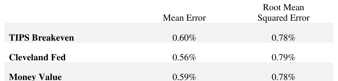
For all its popularity, the 5 year, 5 year forward, a residual of the two uncertain forecasts for 5 and 10 years, is less accurate than for the 10 year alone, which may thus prove to be a better guide for future inflation. Once again, the forecasts with varying methodologies are quite comparable.
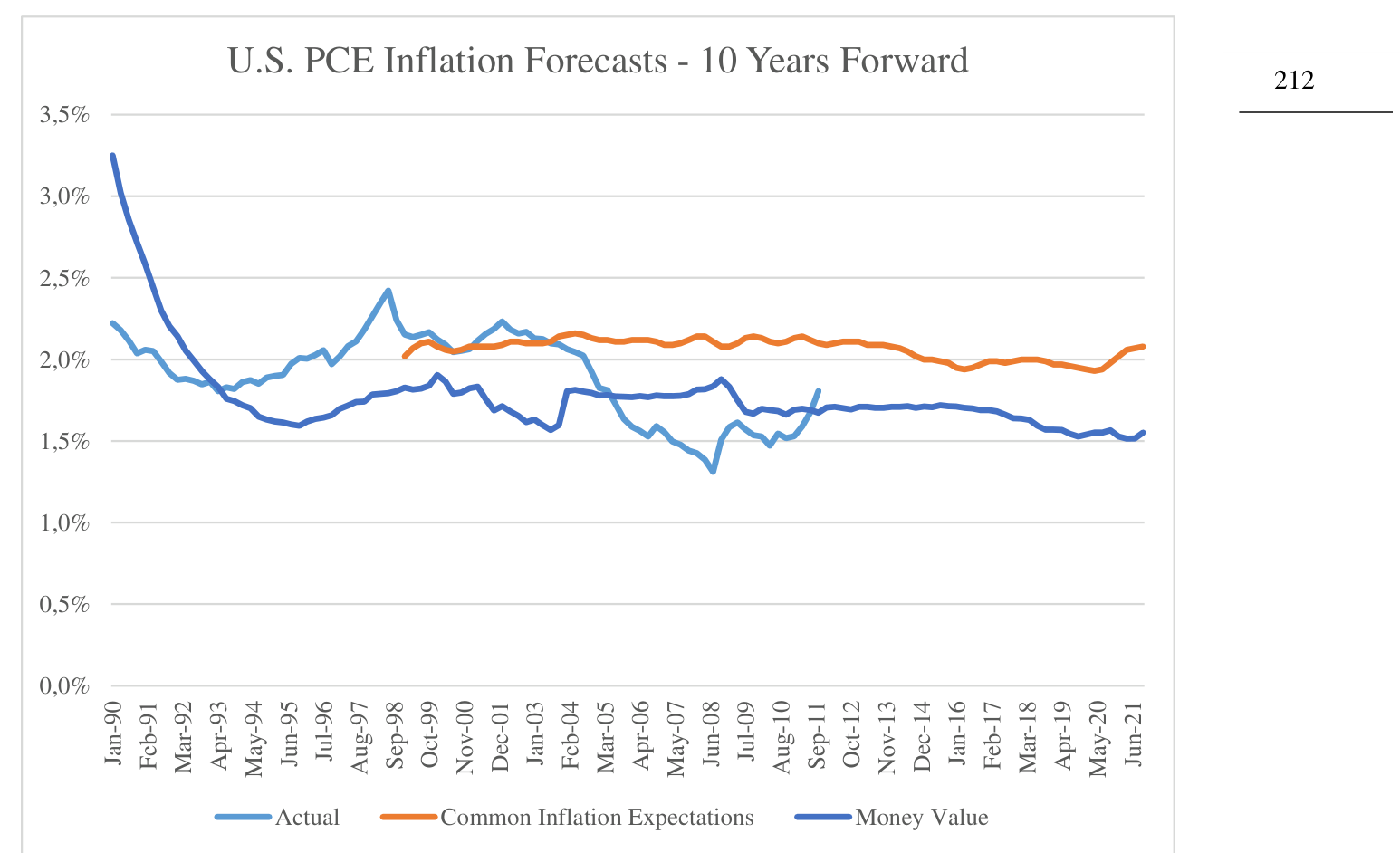
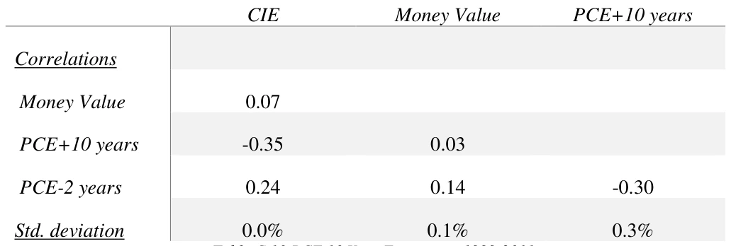
Most of the longer-lived forecasts and financial instruments for inflation rely on the CPI, although PCE figures are a preferred measure for the Fed. 10 year forward PCE inflation forecasts and actuals are shown in Figure C-4 with error statistics in Table C-9 and correlations and variability in Table C-10.
Accessible table text
| — | — | — | — | CIE | — | — | Money Value | — | — | PCE+10 years | — |
|---|---|---|---|---|---|---|---|---|---|---|---|
| — | Correlations | — | — | — | — | — | — | — | — | — | — |
| — | Money Value | — | 0.07 | — | — | — | — | — | — | — | — |
| — | PCE+10 years | — | — | -0.35 | — | — | 0.03 | — | — | — | — |
| — | PCE-2 years | — | 0.24 0.14 -0.30 | — | — | — | — | — | — | — | — |
| — | Std. deviation | — | — | 0.0% | — | — | 0.1% | — | — | 0.3% | — |
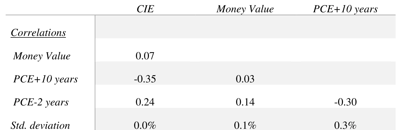
Long-term PCE forecasts are quite accurate, considering the extended term, more so than for CPI estimates of similar length. The alternative forecast methods have low variability and correlation with each other and with inflation measures.
C.2. Short-Term Forecasts
While the primary purpose of this paper is to examine long-term forecasts, short-term forecasts may offer insight into recent forecasting errors, especially for the methods with both long- and short-term forecasts, the Cleveland Fed and Money Value measures, which also were generally most accurate in the long-term. In addition, the Board of Governors Teal (Green) Book is recognized as the forecasting accuracy leader (Ang, Bekaer and Wei 2007).
1 year CPI inflation and forecasts are shown in Figure C-5 with error statistics in Table C-11 and correlations and variability in Table C-12.
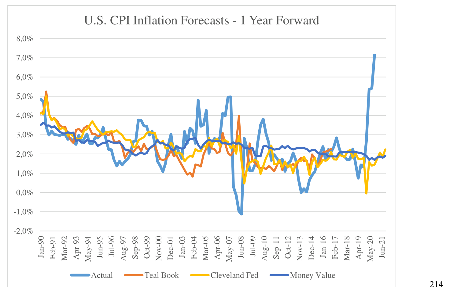
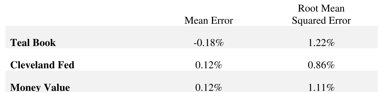
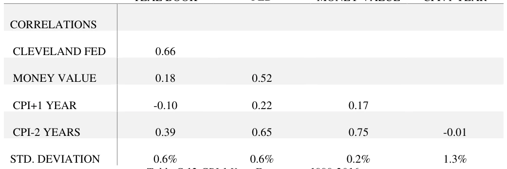
At this short horizon, the Cleveland Fed expectations measure has a decided advantage. It’s noteworthy that forecast errors for 10-year CPI in Table C-5 are 25-50% smaller than for 1 year. It’s evident all forecasts had a big miss with current high inflation, but this is different only in degree from the experience surrounding the Great Financial Crisis or other historical spikes both down and up. The Cleveland Fed measure is highly correlated with alternative methods, but Teal Book and Money Value are not very correlated with each other. All methods are highly correlated with historical inflation and not very correlated with the target 1 year measure, which is significantly more variable than the forecasts.
For 2 year forecasts, the Teal Book data is limited to the second half of each year, but is included for as full a picture as possible. Figure C-6 displays 2 year CPI inflation and forecasts with error statistics in Table C-13.

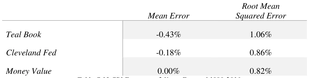
Accessible table text
| Me | — | Root Mean an Error Squared Error | — |
|---|---|---|---|
| — | Teal Book | -0.43% 1.06% | — |
| — | Cleveland Fed | -0.18% 0.86% | — |
| — | Money Value | 0.00% 0.82% | — |


Accessible table text
| Mean | — | Root Mean Error Squared Error | — |
|---|---|---|---|
| — | Teal Book -0.3 | 0% 1.16% | — |
| — | Money Value 0.13 | % 0.84% | — |
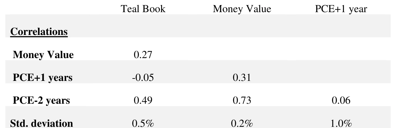
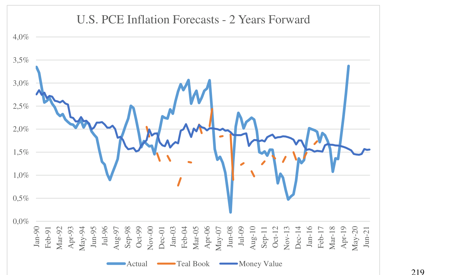
Once again, the PCE forecast errors are somewhat smaller than with CPI, although large spikes above and below forecasts remain. While less volatile than CPI figures, the PCE target remains quite volatile, much more so than the forecasts, which have high correlation with historical figures and lower correlation with each other and with the target PCE figure.
Figure C-8 depicts 2 year PCE inflation and forecasts with error statistics in Table C-16.

Accessible table text
| Me | — | Root Mean an Error Squared Error | — |
|---|---|---|---|
| — | Teal Book - | 0.37% 0.90% | — |
| — | Money Value 0 | .04% 0.64% | — |
The 2 year horizon for PCE inflation has lower errors than at 1 year, and forecasts for PCE outperform CPI projections in Table 16.
C.3. Forecast Characteristics
Forecasts selected for this analysis have widely varying methodologies, yet, in many instances, their results are comparable. All methods had more difficulty capturing shortterm inflation volatility. Long-term forecasts were more accurate with errors of 30-60 basis points providing a reasonable basis for investment and policy decisions.
The purpose of this analysis is not to anoint winners but to understand forecasting dynamics, but the formulaic methods, Cleveland Fed and Money Value, delivered consistently effective projections. CIE also is formulaic but may suffer from being calibrated with survey measures.