 Journal of Global Trade, Ethics and Law
1. Introduction
Previous paper of this series, entitled “Impact of Natural Environment, Regional Integration, and Policies on FDI”, has attempted to provide some empirical evidence on the interrelationships between institutions and economic development from different dimensions (such as economic growth, economic reform and FDI). We essentially try to argue that institutions matter to different economic outcomes. This last paper in series, discusses the role of institutions in cross-country economic performances.
In second paper, entitled “Impact of Institutions and Policy on Economic Growth: Empirical Evidence”, we investigated the effect of institutions on economic growth. The key research questions there are asking primarily asking to do and what institutions matter. Nevertheless, institutions are not production inputs. The mechanism of how they affect output is not demonstrated. The existing literature suggests that institutions may affect productivity, as measured by total factor productivity (TFP) obtained in the standard growth accounting framework. This strand of literature argues that cross-country economic performances are due to different rates of technical change. However, one should note that such TFP obtained as residual from growth accounting implicitly assumes that input allocations are efficient in all economies. This assumption is indeed fairly strong in cross-country analysis.
In this light, this paper proposes to measure technical efficiency instead of TFP growth. We propose that institutional differences affect input allocations, thereby resulting in diverse economic performances across countries. Earlier work by Olson (1996) succinctly points out that an institution is probably one of the most important factors to explain the consistent growth divergence among countries. He argues,
“… Large differences in per capita income across countries cannot be explained by differences in access to the world’s stock of productive knowledge or to its capital markets, by differences in the ratio of population to land or natural resources, or by differences in the quality of marketable human capital or personal culture.”
His empirical findings show that not all poor economies grow faster than rich ones as the theory of convergence has predicted. Even worse, the gap in per capita incomes between the relatively poor and relatively rich countries has increased over time. Prichett (1997) estimates that the proportional gap in GDP per capita between the richest and poorest countries has grown more than five-fold from 1870 to 1990. The proportional gap between the richest group of countries and the poorest grew from 3 in 1820 to 19 in 1998 (see Maddison (2001)).
North (1990) argues that all those determinants of growth – human capital, technological diffusion, and innovations as traditional growth theories suggested – shed no light on the source of growth because they are growing. North and Thomas (1973) note that,
“We are left wondering: if all that is required for economic growth is investment and innovation, why have some societies missed this desirable outcome? … The factors we have listed (innovation, economies of scale, education, capital accumulation, etc.) are not causes of growth; they are growth. … Growth will simply not occur unless the existing economic organization is efficient. Individuals must be lured by incentives to undertake the socially desirable activities. Some mechanism must be devised to bring social and private rates of return into closer parity.”
A better understanding of the source of growth may be efficiency. Countries are “inefficient” in the sense that there is a considerable discrepancy between private benefit and social benefit whenever an economic transaction occurs. 1 Given an institutional arrangement, undertaking an economic activity may be socially profitable, but individuals rationally will not do it if the private cost exceeds the private benefit. Hence, the gains from the transaction cannot be realized. In other words, there actually exists a Pareto optimal (more efficient) outcome, but it cannot be achieved. It is, thus, interesting to investigate how much institutional rigidity could explain the disparity.
Against North’s (1990)’s analytical framework aforementioned, estimating technical efficiency (TE) may help explain the diverse cross-country performances. Hultberg, Nadiri & Sickles (1999), while measuring international TPF growth, also concur that technology diffusion and technical inefficiency are possibly caused by institutional rigidities. Unlike the previous work, on the methodology front, we propose to adopt the stochastic production frontier (SPF) model. This technique allows us to compare the level of technical inefficiency across countries vis-à-vis the global best practice. In addition, the model can also incorporate explanatory factors of technical inefficiency, namely, institutions in our case.
A similar “benchmarking” exercise is not new in cross-country analysis. The standard way is to assume the United States to be the best practice and be used for comparison. These studies then address how far the poor economies are falling behind the best practice. While the key focus of these studies is the comparative performances vis-à-vis the US, time-varying “best practice” is often neglected. In our study, we do not impose such a comparison. Instead, we estimate the world frontier without prior assumptions. In other words, we allow the global stochastic production frontier to shift over time. With regard to the source of technical inefficiency, we consider to test the effects of institutions, human capital and openness. The literature survey we discussed in second paper, has set out the competing debate amongst these three parameters. In an alternative framework as we now propose, we will see if we can contribute some renewed empirical evidence to the debate – i.e. whether institutions, human capital, and/or openness explain crosscountry economic performances, measured in terms of technical efficiency.
In short, there are three research objectives in this paper. Firstly, instead of using TFP measurement obtained from growth-accounting to understand the divergence of crosscountry economic performances, we propose to use the stochastic production frontier model to measure technical efficiency. It does not assume away the inefficiency resulted from input misallocation. Yet, the technique allows us to construct a TFP index if we so wish. Subject to the model specification, the model can also capture any inter-temporal changes of both technological progress and technical efficiency.
1 North and Thomas (1973) suggest that this discrepancy is caused and shaped by the institutional structure, especially when property rights are poorly defined.
Secondly, while understanding the fact that an institution is not a production input, we attempt to investigate exactly what role institutions play in the production process. Based on North’s seminal work on institutions and economic development, we propose to measure the impact of institutions on cross-country technical efficiency, i.e. the efficiency of input allocations across economies.
Thirdly, we revisit the competing debate between the institutional view vis-à-vis the impacts of openness and human capital on economic development. From our empirical results, we will evaluate whether cross-country technical efficiency can be explained by any or all of these three factors.
This paper is organised as the following. First, we will survey the previous relevant literature of the effects of institution, openness, human capital on productivity in Section 2. We outline the fundamental concepts of stochastic production frontier in Section 3. The model we adopted for estimation is further elaborated in Section 4. Data used are discussed in Section 5. Section 6 presents the estimation results. We conclude in Section 7.
2. Literature Survey: Institutions, Openness, and Human Capital as Efficiency Sources
Productivity is the source of growth and deep determinants of cross-country economic development. Sources of TFP growth are considered to provide an opportunity for enhancing general welfare of the society. The large and growing literature consistently provides support to the claim that productivity, rather than factor accumulation, is the key explanation for international income disparities.
Productivity, frequently measured in terms of TFP, can be further segregated into technical progress and efficiency change. The former represents the country’s knowledge as to how factors of production can best be combined. This can be the results of innovations or learning and imitation. Efficiency, on the other hand, represents how effective a country’s factors are actually used. A distinct point between the two dimensions worth noting is that the presence of obsolete production techniques does not necessarily imply a technology gap. In fact, it may reflect a situation in which producers are discouraged from adopting best-practice techniques. The presence of suboptimal technologies may be a symptom of poor efficiency instead of resulting from unavailable technology.
Most of the existing empirical literature focuses on the source of TFP. From these empirical studies, nevertheless, we are unable to tell whether the differences in crosscountry TFP growth are the results of technical change or efficiency change. In fact, there are views that technology is quite readily available, especially in this globalised era. The differences in economic performances across countries are believed to be the results of technical inefficiency.
Efficiency becomes more prominent in recent studies of economic development. Echoing the view of North on the role of efficiency differences as the source of diverge economic performances, Parente & Prescott (2005) lately also develop a theory to explain international income levels. From a historical perspective, they develop a relative efficiency theory of economic development to explain the evolution of international income levels in the last millennium.
The essence of their theory provides a sensible link between efficiency and institutions. They argue that a country starts to experience sustained increases in its living standard when production efficiency reaches a critical point. Countries reach this critical level of efficiency at different dates not because they have access to different stocks of knowledge, but rather because they differ in the amount of society-imposed constraints on the technology choices of their citizenry. Their theory argues that country-specific TFP, which they refer to as a theory of relative efficiency, is a consequence of policy differences. Their theory predicts that after a country reaches a critical point of efficiency, it begins to grow. Its income gap with the leader eventually stops increasing. Nevertheless, to reduce such a gap (i.e. to improve efficiency), the late starter has to use resources in the modern production function by making improvements in its policies and institutions. Growth miracles, as observed in Japan, South Korea, and Taiwan, are also the results of large increase in a late starter’s relative efficiency. Parente and Prescott (2005) provide an essential theoretical foundation of our empirical investigation, even though technically speaking, we adopt a more refined measurement of cross-country technical efficiency instead of TFP, which we will discuss in the next section.
While efficiency is essential to close income gap, it is natural henceforth for us to explore the potential factors determining efficiency.2 Sources of international technical efficiency are not frequently explored. Therefore, we will consider key factors previously examined in the productivity literature and see if they are applicable in our context. In our study, we consider three key dimensions: (i) human capital; (ii) openness, and (iii) institutions and macroeconomic policies. We will review the arguments and the empirical evidence put forth in the literature in turn.
2.1. Human Capital
Human capital enhances productivity in two possible ways. On one hand, it improves average labour productivity. On the other hand, it strengthens the innovation capacity and promotes technological progress. When summarising recent empirical work on the relationship between human capital and economic growth, Isaksson (2002) concludes that empirical results are diverse with respect to statistical significance (significant or not), magnitude (small or large), and sign (positive or negative) of the estimated parameter. Incorporating human capital or not in the production process produces mixed and somehow puzzling empirical results. For relatively rich countries, human capital is important, while its effect is negative for relatively poor ones.
2 See Isaksson (2007a) for a comprehensive survey on the sources of productivity.
In terms of empirical evidence, Benhabib & Spiegel (2005) refine their own established model in Benhabib & Spiegel (1994) by allowing for different functional forms for predicting TFP growth. Studying 84 countries between 1960 and 1995, they find a positive role for human capital as an engine of innovation, as well as a facilitator of TFP catch-up. The predictive capacity of the model seems very good because 22 of 27 countries that were forecast to fall behind did in fact do so.
Along the line of Acemoglu, Aghion & Zilibotti (2006), Vandenbussche, Aghion & Meghir (2006) specifically develops a theoretical model to understand the ambiguous effect of human capital on technological improvements. They argue that labour composition determines the form of technological improvements, either innovation or imitation, in an economy. Innovation requires relatively more skilled labour, whereas unskilled labour better endogenous labour allocations across these two activities. The authors opine that both the economy’s distance to the technological frontier and the composition of its human capital suit imitations.
A country’s level of technological development therefore depends on the determined economic development. Skilled labour (i.e. human capital) is growth-enhancing only when the country is proximate to the frontier.
2.2. Openness: FDI, Trade, and Financial Integration
Isaksson (2007a) reckons that knowledge is only created by a few leading technologically advanced developed economies. Elsewhere, technology is just being acquired. Identifying the channels through which technology can be transferred effectively is thus important. Amongst different forms of technology transfer, international trade, in particular imports, and FDI have a relatively high knowledge content embodied. Thus understandably openness is treated as the source of learning. It then presents indirect effects on productivity. Trade liberalisation may lead to increased competition and reduce a firm’s X-inefficiency. Foreign competition may also lead domestic producers to expand or cease operations to improve overall efficiency. As Tybout (1992) recognises demand shifts accompanied by trade liberalisation, market flexibility (entry and exit), and the nature of competition may all affect the net effect of liberalisation on TFP.
FDI is also generally viewed as the key channel for the transfer of advanced technology from industrialised to developing economies. It is also believed to generate positive externalities in the form of knowledge spillovers to domestic firms. However, foreign capital may also crowd-out domestic investment, replace domestic production, and reduce competition. Hence, the net effect of technology transfer and efficiency gain as a result of openness is not definite.
Empirical studies of whether FDI spurs productivity is mostly micro-level in nature. Granér & Isaksson (2001) find that both mixed and pure foreign ownership is positively correlated with productivity growth. Keller (2004) uses case studies to show large positive FDI spillovers. On the contrary, Aitken & Harrison (1999) show a negative effect of FDI on productivity among Venezuelan plants, explaining that foreign firms recruit the most skilled workers and hence deprive domestic plants of their services. Cases in Hanson (2001) also show that spillovers from foreign capital are limited.
Also using SPF, Nourzad (2008) investigates the effect of FDI at macro-level technical inefficiency. His results suggest that increased FDI increases potential output in both developed and developing countries with the effect being more profound in the former. Furthermore, FDI reduces technical inefficiencies in developed economies, but not in those developing ones.
In a nutshell, these empirical results point to a general conclusion that FDI only has a positive impact on TFP growth in industrialised countries, while such positive results are harder to observe in developing countries. Isaksson (2007a) explains that it may be because technology transfer can be costly. Different absorptive capacities across countries may also help explain such a pattern.
This also suggests that openness and human capital may have to interact together to have any impact on productivity. Mayer (2001) attempts to interact technology transfer with human capital in a cross-country growth regression. The proxy of absorptive capacity is captured by an interaction term between human capital and imports of machinery and equipment (as percentage of GDP). During the studied period of 1970-1990 in 53 developing countries, the results show that the interaction term has a significant coefficient, meaning human capital is significant for technology adoption.
Separately, Isaksson (2001) uses data on 73 countries between 1960 and 1994 and shows that trade can be viewed as a significant carrier of knowledge or technology unless the recipient countries have the necessary level of human capital. Miller & Upadhyay (2000), covering 83 countries over the period 1960 and 1989, present a statistically significant impact of the interaction of exports and human capital on productivity. More specifically, they argue that the interactive term works differently in countries with different income levels. At low-income levels, human capital is negatively associated with TFP growth, while for middle- and high-income countries the effect is positive. Nevertheless, in the case of Harrison (1996), while analysing 51 countries between 1960 and 1987, shows that such interaction terms are seldom statistically significant.
In sum, empirical studies prevalently show that openness has positive effects for industrialised countries, while not necessarily for the case of developing countries. Again, this leads one to suspect that institutional quality may affect absorptive capacity, which in turn affects productivity growth. Although the trade channel could in principal facilitate technology transfer, the absorptive capacity of the recipient country, mainly depending on human capital and capital intensity, determines the magnitude of technology transfer.
Other than trade openness and FDI, financial openness also raises the issue of financing capital accumulation, which may have repercussions for productivity growth (Isaksson (2007a)). In economies where the financial system is well developed, investment opportunities can readily be seized, resources are more likely to be allocated optimally. Specialisation can thus be promoted. However, in developing countries with less sophisticated financial systems, firms may have to rely on retained earnings for investment or forego the opportunity. Financial constraints therefore may prevent poor countries from taking full advantage of technology transfer. Financial repression, often exemplified by negative or artificially low real interest rates, thwarts incentives to save. It also distorts the efficient allocation of savings into investment and hence brings negative effect on TFP growth.
The association between financial development and productivity growth receives great research interests lately. Fisman & Love (2004) study the relationship between industrial growth (covering 37 developed and developing industries with good growth opportunities in 42 countries between 1980 and 1990) and financial development. Based on Rajan and Zingales (1998)’s framework, they conclude that financial development spurs productivity growth. At the macro-level, Aghion, Howitt, and Mayer-Foulkes (2005) study 71 countries between 1960 and 1995. They find that financial development is a threshold variable, which affects convergence mainly through TFP growth rather than capital accumulation.
Recent studies also suggest that there are many channels through which financial openness can have a positive impact on productivity growth. For example, Kose, Prasad & Terrones (2008) argue that financial openness could have a positive impact on TFP growth because they lead to more efficient resource allocation as Mishkin (2006) suggests. More specifically, the authors find that de jure capital account openness has a robust positive effect on TFP growth. The effect of de facto financial integration, measured by the stock of external liabilities to GDP, on TFP growth is less clear. FDI and portfolio equity liabilities boost TFP growth while external debt is actually negatively correlated with TFP growth. They explain that financial openness might affect the return to capital, thereby leading to changes in the entry and exit decisions of firms/plants. Aggregate factor productivity will increase because new plants are more productive than exiting plants. This reallocation from less productive to more productive plants would ultimately increase total factor productivity with no significant gains in employment. These productivity gains from both learning and selection effects may also have to spread over longer periods. It may turn out the net effect on TFP seems insignificant.
2.3. Institution and Macroeconomic Policies
The institution view argues that differences in efficiency across countries are the results of the underlying market-friendly institutions, including the set of formal and informal constraints that shape an individual’s ability to act productively and cooperatively in the society. The role of institutions ensures efficient allocation of resources across sectors. On the other hand, policy instruments may also compensate for weak underlying institutions.
According to Isaksson (2007a)’s survey, the existing literature generally highlights three main institutional issues, namely, (i) enforcement of property rights (encourages investment), (ii) constraints on the actions of elitist, political and other groups with power (thus reduce risks of expropriation of incomes and others’ investments), and (iii) equal opportunity for broad segments of society (e.g. enhanced investment in human capital and participation in productive activities). Theories argue that better security of property rights creates more incentives for savings and investment, leading to TFP growth. As defined in second paper of this series, we consider institutions as a measure composed of economic and political institutions, macroeconomic policies and regulations.
Openness, policy and institution are three typical deep determinants of productivity growth. Empirical studies frequently test their competing roles simultaneously. Alcalá & Ciccone (2004) claim that the way to measure trade matters to the empirical results. They use real openness (i.e. as predicted trade shares estimated based on gravity model), instead of trade share to GDP, and find a strong positive and statistically significant effect on productivity. Their results remain robust after controlling for geography and institutional quality. Nevertheless, Bosworth & Collins (2003), in respect of 84 countries during 1960-2000, show that trade renders insignificant effect in the presence of institutional quality. One possible explanation is that macro studies mask the heterogeneity bias. In reality, trade liberalisation might only benefit large firms. The removal of protective measures could be harmful for smaller enterprises. The net effect may therefore become insignificant.
Hall & Jones (1999), as previously discussed in second paper, strongly believe that the primary and fundamental determinant of a country’s long-run economic performance (as measured by output per worker) is its social infrastructure. They argue that differences in social infrastructure cause large differences in capital accumulation, educational attainment and productivity, resulting in huge income disparities across countries. Nevertheless, Glaeser, et al. (2004) suggest that human capital may be more fundamental.
More specifically in terms of political regime, Przeworski & Limongi (1993) appear to favour dictatorships in terms of mobilising savings. However, the authors also recognise that methodological limitations, such as endogeneity problem of institutions and economic development, may hamper one to draw reliable conclusion. In the empirical work of Ulubasoglu & Doucouliagos (2004), their results support that both political and economic institutional variables are important to TFP. Their results show that higher levels of democracy have a positive and statistically significant effect on TFP and human capital. Using both economic and political freedom variables in the estimations, their results show that these two variables have positive effects on TFP.
Loko & Diouf (2009) consider altogether the effects of macroeconomic stability (in terms of inflation), FDI, trade openness and business environment on TFP in Maghreb countries in a dynamic panel data setting. They attempt to test the complementary effect of policies to trade openness following Chang, Kaltani, & Loayaza (2005). Their results demonstrate that macroeconomic stability, openness and the level of education are all important for productivity growth. In particular, higher inflation hampers productivity gains significantly, confirming the negative impact of macroeconomic instability. Notwithstanding, their three alternative measures of institutions – the degree of regulation of credit, labor, and business; law and order; and the economic freedom index – all point to the importance of institutions to high TFP growth.
On regulations, its effect on productivity appears to be straightforward. A less regulatory environment is conducive to a more competitive environment, thereby promoting productivity and efficiency growth. Stringent regulation is a hindrance to technology adoption and innovation, possibly because it reduces competitive pressures, technology spillovers and the entry of new high-tech firms. Crafts (2006) argues that regulation can be thought of as rules imposed by the State. Such rule can be used to correct market failures through acting to reduce the costs of negative externalities or imperfections of information by providing insurance or public goods. However, such action also typically imposes costs on the private sector. So there is a danger of excessive regulation where additional costs exceeded extra benefits. All in all, the effectiveness of regulation depends on enforcement as well as legislation.
One of the empirical studies investigating the effect of regulation and the institutional environment on productivity is Scarpetta et al. (2002). They note that, across OECD countries, growth paths have become increasingly disparate in the past decade. They suggest two possible reasons: (i) differences in productivity patterns of certain high-tech industries and (ii) differences in the adoption of information and communications technology (ICT). They find that stringent regulatory settings in the product market negatively affect TFP. In addition, labour market regulations that induce high hiring and firing costs also have a negative effect on TFP. In particular, such negative effects are worse for firms in countries which are far from the technological leader.
Based on the World Bank’s investment climate survey in five transition economies –the Kyrgyz Republic, Moldova, Poland, Tajikistan and Uzbekistan, Bastos and Nasir (2004) similarly conclude that productivity differences across countries can be explained largely by differences in the investment climate, e.g. policy, institutional and regulatory environment, in which businesses operate. In particular, competition seems to be the most important factor behind productivity performance, followed in the second place by infrastructure, while rent predation (e.g. corruption) occupies the third place. To sum up, we have reviewed some of the recent theoretical and mostly empirical literature, discussing the sources of productivity in this Section. The deep determinants of productivity include human capital, openness and institutions. Studies examining the effects of these factors alone do not bring conclusive evidence. Conflicting results are often found between developed and developing economies. The literature suggests that one would expect the determinants of productivity growth in technological leaders and recipients to be different (i.e. their relative positions in the global technology frontier matter). However, exactly how much the less developed economies are falling behind the technological leaders is not clear. By its very own nature, TFP per se does not allow us separately to understand how technical change and efficiency change take place. We fail to know if the economy does not “catch-up” because of the barriers of technological adoption or inefficient allocation of resources. In this regard, we consider an alternative measurement technique – i.e. stochastic production frontier – to estimate the efficiency change across countries.
3. Fundamentals of Stochastic Production Frontier (SPF)
To estimate the efficiency of production, Farrell (1957) suggests that the efficiency of an individual cross-section, say a firm, consists of two components: (i) technical efficiency, measuring the ability of a firm to obtain maximal output from a given set of inputs; (ii) allocative efficiency, measuring the ability of a firm to use the inputs in optimal proportions, given their respective prices. In a cross-country context, our primary research interests lie on the measurement of technical efficiency. In this section, we will discuss the basis of our estimation methodology, i.e. stochastic production frontier (SPF), and present a brief survey of some of its applications. Generally speaking, efficiency measurement relies on estimating a “global” production frontier of a number of crosssections. Data envelopment analysis (DEA) and stochastic frontiers are two convention methods for such purpose. Coelli, Rao & Battese (1998) compare the merits and characteristics between these two, which are summarised in Table 1 below:
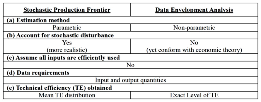
Source: Coelli, et al. (1998)
As compared to DEA (also known as deterministic frontiers), although it ignores the stochastic effect on production frontier, they are more consistent with economic theory. DEA is also more advantageous in terms of obtaining the exact measure of technical inefficiency for each observation instead of its distribution. However, its chief disadvantage is that they are bound to be confounded by statistical ‘noise’, whereas stochastic frontiers are more realistic, at least in terms of econometrics. Moreover, due to its non-parametric approach, DEA is more sensitive to outliers. Since this study is primarily empirical in nature, the readiness of hypothesis tests developed for SPF provides an added advantage for us to choose SPF over DEA for our estimation.
3.1. Basic Framework
SPF is an estimation of a “global” production frontier of a number of cross-sections while incorporating stochastic assumptions. Based on this concept of productivity, we can measure the economic performance of each country relative to the world’s best possible output given the available resources and technology at each time period. This comparative measurement of economic performance against the world production frontier is regarded as technical efficiency.
SPF assumes a mixture of one-sided and two-sided (e.g. normal) errors. The error term is composed of two parts. The one-sided component captures the effects of inefficiency relative to the stochastic frontier. The two-sided component permits random variation of the frontier across cross-sections, and captures the effects of measurement error, other statistical ‘noise’, and random shocks outside the cross-sections’ control.
In a nutshell, the measurement attempts to capture that given the quantities of a list of inputs, there is a maximal possible output. However, this maximum level is random (to be precise, which is randomly distributed as a function) rather than exact. This assumes that some inputs or external effects have maximal possible effects, but others have potentially unbounded effects, e.g. weather. In general form, a production function can be specified as followed:

where i denotes the i-th cross-section. y denotes the unit of output. a measures the technology parameters. x is a (1 x k) vector of inputs of production and other explanatory variables and β is a vector of coefficients of inputs to be estimated. Rewriting eq.(1) in log-form gives:

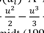

Assume 𝑣 ∼𝑖𝑖𝑑 𝑁 (0 , 𝜎2) is a stochastic error independently distributed of u . It accounts for the measurement such as the effects of weather, strikes, luck etc on the value of the output variable together with the combined effects of unspecified input variables in the production function. Therefore it is simply treated as random disturbances.
u, on the other hand, is assumed to be a non-negative random variable associated with technical inefficiency of production and is again assumed to be independently distributed. Among the different cross-sectional SPF models, there are a number of specifications of u commonly proposed. For examples, Aigner, et al. (1977) and Meeusen and Broeck


By definition, TEi takes a value of zero to one.
Eq.(4) suggests that if 𝑢𝑖 = 0, then 𝜀𝑖 [sum of 2-sided errors, 𝑢+ 𝑣] is vi, the error term is symmetric, and the data do not support a technical inefficiency story. However, if 𝑢𝑖 > 0, then 𝜀𝑖 = 𝑣𝑖 − 𝑢𝑖 is negatively skewed, and there is evidence of technical inefficiency in the data. In other words, the production process is subject to two random disturbances, namely u and v. The frontier is stochastic with random disturbance of 𝑣𝑖 ≤𝑜𝑟≥0. Technically speaking, we can estimate the variances of 𝑣𝑖 𝑎𝑛𝑑 𝑢𝑖 for each cross-section.
3.2. Some Applications of SPF
There are numerous studies using the stochastic frontier approach for various applications, mostly for firm-level and industry-level analyses. Models derived from different assumptions and techniques have been extensively employed. The technique was initially developed for applications at firm-level and industry-level studies, especially on agricultural economics (such as in Battese & Coelli (1992) and Battese & Coelli (1995)) concerning the measurement of inefficiency across different producers. Meeusen & Broeck (1977) were probably among the first to test their model on several manufacturing industries. After developing panel data stochastic frontier models,4 recent work like Paul, Johnson & Frengley (2000), Bhattacharyya, Bhattacharyya & Mitra (1997), Mahadevan (2002) and Kruger, Canter & Hanusch (2000) deploy several variations of panel data SPF models for their micro-level studies.
Empirical applications of SPF have been reasonably extended to country-level data. Macro-level work mostly intends to estimate the efficiency levels across countries under different political environments and/or regime changes. In particular, the political changes that took place in Eastern Europe facilitate the comparison of efficiency levels in market-oriented vis-à-vis planned economies. For example, Koop, Osiewalski & Steel
3 We do not aim at providing a survey on various SPF models for cross-sectional analysis since we will carry out panel data analysis. For further reference, Coelli, et al. (1998) and Kumbhakar and Lovell (2000) provide excellent surveys of different SPF models.
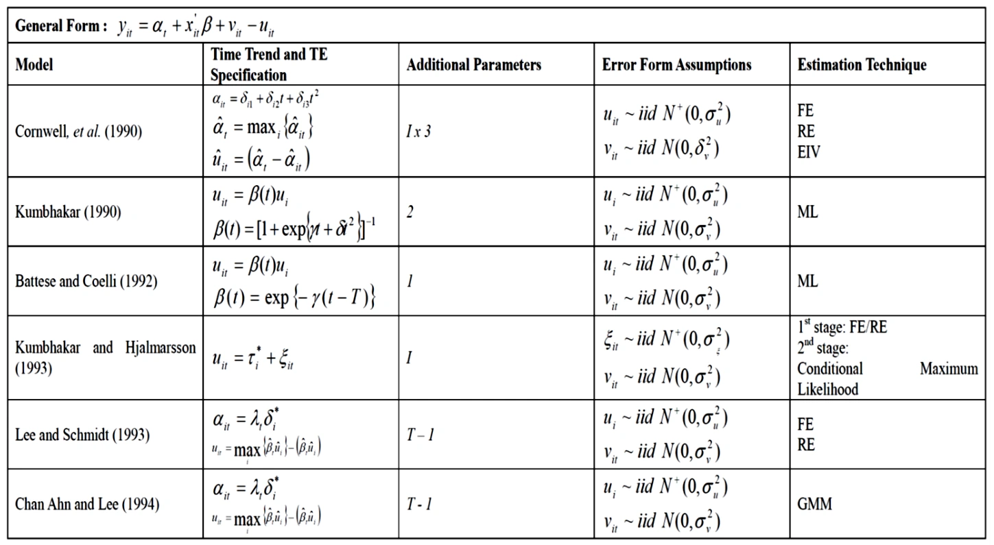
4 Among others, more prevalently used panel data SPF models include Schmidt and Sickles (1984), Cornwell, Schmidt, and Sickles (1990) and Battese and Coelli (1992) and Battese and Coelli (1995). See Appendix Section A.3 for details.
- initially focus their measurement exercise on 17 OECD countries. Koop, Osiewalski & Steel (2000) extend further the measurement and make special reference to Poland and Yugoslavia in comparison to 20 Western economies.
Moroney & Lovell (1997) share a similar interest and measure the relative efficiencies of 7 transition economies in comparison to other Western economies. Klein & Luu (2003), on the other hand, use the indices of economic freedom and political constraints as independent variables for explaining inefficiencies in 39 countries from 1975 to 1990. Their results show that technical efficiency relates positively to policies supporting laissez-faire and political structures that promote policy stability. Adkins et al. (2002) on the other hand investigate the impact of economic freedom on promoting efficiency.
However, SPF models are mostly applied to mere measurements of technical efficiency. The sources of technical inefficiencies are not considered and/or incorporated in these models. To incorporate exogenous variables to explain the sources of technical inefficiency, some of the researchers approach the problem using a 2-stage approach. In the first stage, they use the aforementioned SPF models to obtain the technical inefficiency measures, typically by maximum likelihood estimation (ML). In the second stage, the estimated technical inefficiency is treated as dependent variables to be regressed on a vector of explanatory variables in the form such as


In some cases, it is recognised that since the dependent variable u lies between 0 and 1, OLS estimates cannot be used. Instead, an estimation technique such as Tobit for limited dependent variable estimation is employed.
Amongst various studies of such kind, Liu, Liu & Wei (2001) make special reference to trade openness in the case of India and China. They first employ a dynamic approach to the estimation of a production function and then in the second stage, technical efficiency is treated as a dependent variable. Their key results show the relationship of trade openness and their relative technical inefficiencies for the case of India and China.
Although it is fairly often that early literature associating technical inefficiency and its sources uses the aforementioned 2-stage approach, estimations of such kind are fundamentally problematic in terms of econometrics. As Battese & Coelli (1995), Coelli et al. (1998) and Kumbhakar & Lovell (2000) argue, such an approach has at least 2 obvious flaws. Firstly, 2-stage estimations ignore the fact that SPF models in the first stage have assumed a particular distribution of the level of technical inefficiency, u. In other words, u is frequently assumed to be an independent random variable with particular distribution. This contradicts with the second stage, where the predicted mean efficiencies are assumed to have a functional form of z_i. It is thus statistically inconsistent to assume u again at the second stage with any form of specification.
Secondly, the 2-stage approach imposes a restricted assumptions that z_i are uncorrelated with xi, the production inputs. Otherwise, the estimates obtained in the first stage are biased due to omitted variables. The biased estimates of technical inefficiency being used as dependent variables inevitably undermine the validity of results obtained in the second stage of estimation.
Since our primary research interest of this paper is to investigate whether institutions can explain the cross-country technical inefficiencies, SPF models that allow us to incorporate exogenous explanatory factors are essential. While recognising the inadequacies of using a 2-stage approach as in the current literature, we will employ an alternative approach to tackle the problem of such kind. The models we use will be discussed in more details in the next section (4).
3.3. General Critics on SPF
We do not intend to argue that SPF models are strictly superior to DEA. Indeed, we fully recognise the limitations of this methodology. As Førsund, Lovell & Schmidt (1980) point out, even though SPF captures a more realistic world, unfortunately there is no way of determining whether the observed performance of a particular observation compared with the deterministic kernel of the frontier is due to inefficiency or to random variation in the frontier. This constitutes the main weakness of the SPF model – i.e. it is not possible to decompose individual residuals into their two components, and so it is not possible to estimate technical inefficiency by observation. What we are estimating is simply the mean inefficiency over the sample, but not its “true” value.
Secondly, Coelli et al. (1998) realise that when using the stochastic frontier approach, the specification of the functional form of the production function matters for the results. Monte Carlo simulation results from Giannakas, Tran & Tzouvelekas (2003) indicate that the bias in the mean efficiency measures from stochastic frontier methods due to misspecification of functional form is sizeable. It can suggest a high level of inefficiency (10-30%) of output for the most efficient producers. As Ravallion (2003) also criticises; the approach using non-parametric methods is more preferable in some cases, especially when measuring social efficiency using social indicators. Parametric estimation, like SPF, is very sensitive to outliers and one must assume a continuous frontier. Likewise, the distribution of the inefficiency term also has to be specified.
The stability and reliability of the results are also concerns too. The measured efficiency is only relative to the best cross-section in the sample. Including extra crosssections may alter the efficiency scores. Furthermore, measurement error and other noise may influence the slope and position of the frontier. Not surprisingly, measurement errors and outliers will likewise influence results significantly. In our estimations, we attempt to alleviate some of these problems by using a reliable source of data to minimize the measurement errors as far as possible.
4. Model Estimation and Specification
There are primarily four dimensions of SPF models developed and could be considered in our case. These include cross-sectional versus panel data models and with or without assuming time-varying technical efficiency. We will consider the most flexible forms of SPF models – i.e. panel data model with time-varying technical efficiency. The availability of panel data generally implies that there is a large degree of freedom for estimation. It also permits the simultaneous investigation of both technical change and technical efficiency change over time.
There is also one added advantage of using panel data SPF models. Specification of the error term and the inefficiency term is one of the major challenges of using stochastic production frontier estimation. However, Schmidt & Sickles (1984) show that when panel data are available, assumptions on the distribution of technical inefficiency could be relaxed since the parameters can be estimated using the traditional panel data methods of fixed-effects estimation or error-components estimation. Measuring the technical efficiencies of the sample can be rather straightforward hereafter as they can be obtained relative to the most efficient one(s). This view is also shared by Kumbhakar & Lovell (2000).
The basic framework of panel SPF model is generally similar to the cross-sectional one set out in Section 3.1. Appendix Section A.3 summarises some key panel time-varying SPF models, which are often used in the existing literature.
4.1. Battese and Coelli (1993) and (1995) Model
Our model of estimation is based on the Battese & Coelli (1993) and Battese & Coelli (1995) model. The key advantage of their model is that it allows incorporating the technical efficiency model in the stochastic production frontier estimation to perform a one-stage simultaneous estimation.
Following eq.(2), the stochastic production frontier in panel data form is defined as:


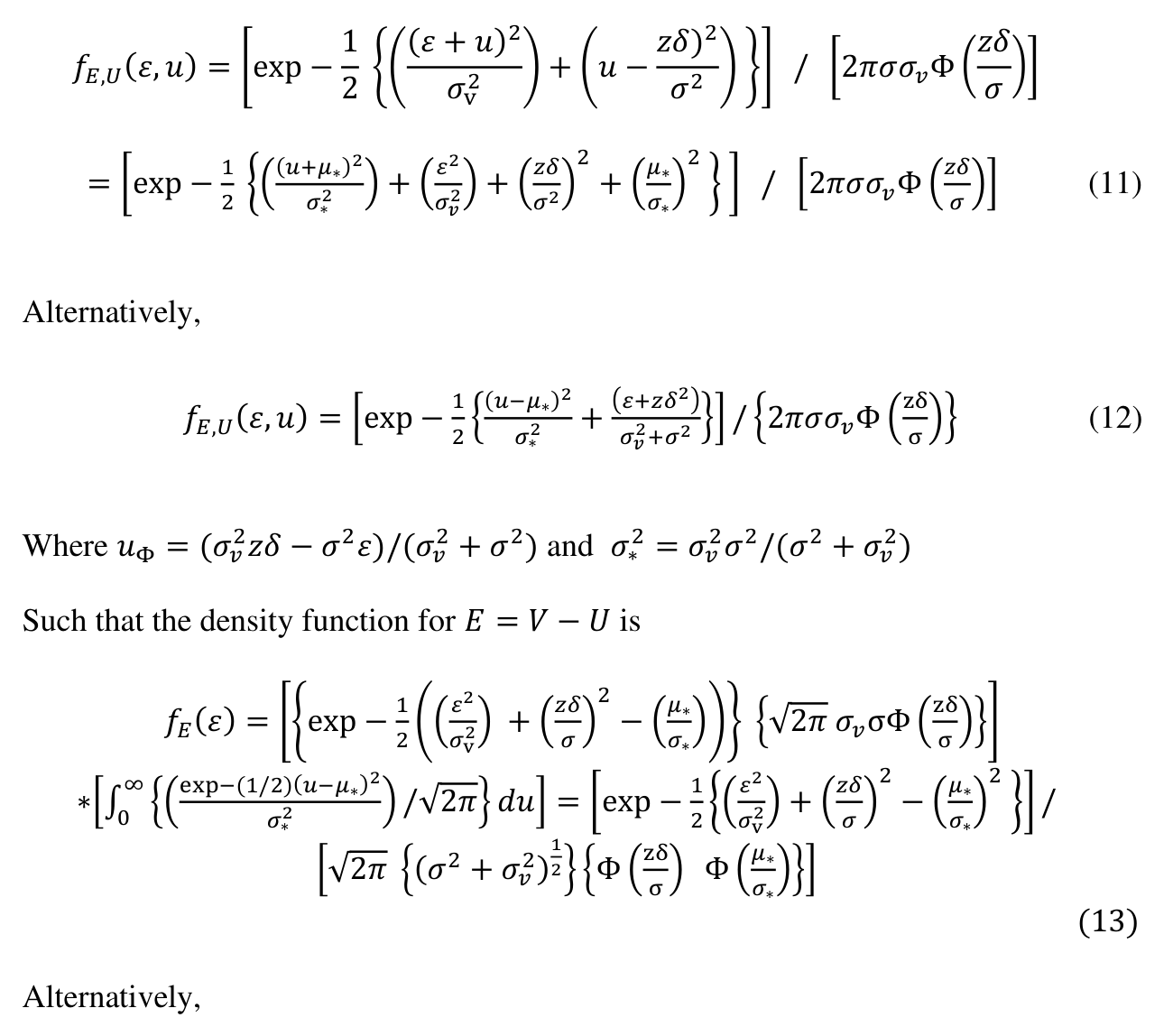
Were Wit is a random variable and is defined by the truncation of the normal distribution with zero mean and variance σ2 and 𝑊𝑖𝑡 ≥𝑧𝑖𝑡 𝛿. Technical inefficiency (𝑈𝑖𝑡 ) is assumed to be independently distributed for all t and i and is obtained by truncation (at zero) of the normal distribution with mean 𝑧𝑖𝑡 𝛿 and variance vector of country specific institutional environment which may vary over time. 𝛿 is an (m x 1) vector of unknown coefficients. Technical efficiency of production can be defined as:
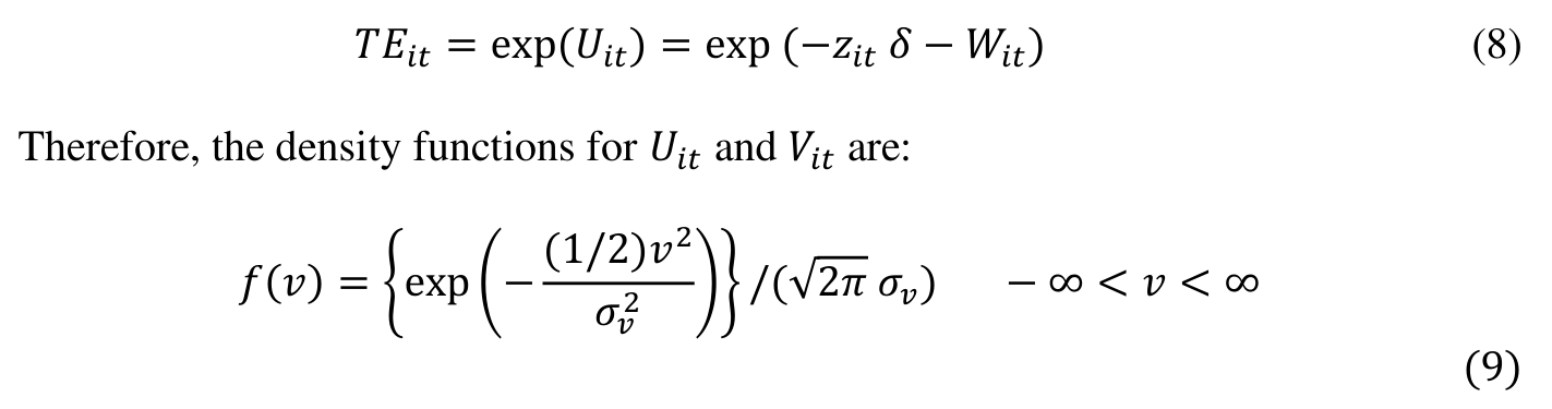

![1 2 {Φ (𝑧𝛿 𝜎) / (Φ (𝜇∗ 2 + 𝜎2)}] / [ √2𝜋 (𝜎2 + 𝜎𝑣 2 (𝜀−𝑧𝛿)2/(𝜎𝑣 2) ))}] 𝜎∗ (14)](/static/article-media/cross-countries-economic-performances-spf-approach/equation-015.png)
![The conditional density function for U given 𝐸= 𝜀 is thus (𝑢−𝜇∗)2 1 𝜇∗ 𝜎∗)] 𝑓𝑈|𝐸=𝜀(𝑢) = [exp − 2 { 𝜎∗2 } ] / [√2𝜋𝜎∗Φ (](/static/article-media/cross-countries-economic-performances-spf-approach/equation-016.png)
(15)
![Conditional expectation of 𝜀−𝑈 given 𝐸= 𝜀 is Φ{(𝜇∗ /𝜎∗)−𝜎∗} 1 𝐸(𝜀−𝑈|𝐸= 𝜀) = [exp (−𝜇∗+ 2) ] [ 2 𝜎∗ Φ(𝜇∗/ 𝜎∗) ]](/static/article-media/cross-countries-economic-performances-spf-approach/equation-017.png)
(16)
Such that the density function for Yit in eq. (6) can be derived from eq. (14):
![1 2 { Φ(𝑑𝑖𝑡) 1 𝜎𝑣2+𝜎2 } ] / [ √2𝜋 (𝜎2 + 𝜎𝑣 2) ∗)} ] (17) 𝑓𝑌𝑖𝑡(𝑌𝑖𝑡) = [𝑒𝑥𝑝− 2 { Φ(𝑑𝑖𝑡](/static/article-media/cross-countries-economic-performances-spf-approach/equation-018.png)
![2 + 𝜎2) ∗= 𝜇𝑖𝑡 ∗/𝜎∗ and 𝜇𝑖𝑡 ∗= [𝜎𝑣 2𝑧𝑖𝑡𝛿−𝜎2(𝑌𝑖𝑡−𝑥𝑖𝑡𝛽)]/(𝜎𝑣 Where 𝑑𝑖𝑡= 𝑧𝑖𝑡𝛿/𝜎 , 𝑑𝑖𝑡](/static/article-media/cross-countries-economic-performances-spf-approach/equation-019.png)
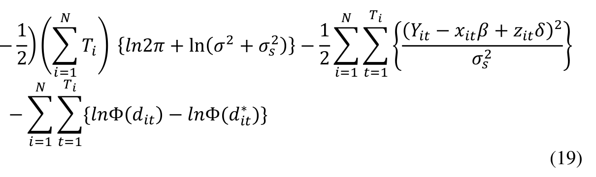
The logarithm of the likelihood function for the sample observations y is:



![∅(𝑑𝑖𝑡) ∅(𝑑𝑖𝑡) 1 1−𝛾 𝜎∗)} ] . 𝑧𝑖𝑡 𝑇𝑖 𝑡=1 𝑁 𝑖=1 1/2)} − {( 𝜎𝑠2 ) + {( Φ(𝑑𝑖𝑡)) . ( Φ(𝑑𝑖𝑡)) . ( (𝛾𝜎𝑠2) (21)](/static/article-media/cross-countries-economic-performances-spf-approach/equation-024.png)
𝜕𝐿∗

𝜎𝑠2)
] 𝑖=1 𝑡=1
(22)

Where is the density function for the standard normal random variable. The necessary condition for maximizing the log-likelihood function is that these partial derivatives equal 0.


Respectively. The OLS estimates are used for the remaining parameters in 𝛽. 3) The values selected in the grid search are used as starting values in an iterative procedure to obtain the final maximum likelihood estimates.
4.2. Post-estimation Test
The one-sided generalized likelihood-ratio test (hereafter called LR-Test) can be used for hypothesis testing. This aims at providing a statistical test of the goodness-of-fit between two models. In short, a relatively more complex model is compared to a simpler model to see if it fits a particular dataset significantly better. If so, the additional parameters of the more complex model are often used in subsequent analyses. The LR-Test is only valid if it is used to compare hierarchically nested models. That is, the more complex model must differ from the simple model only by the addition of one or more parameters. Further addition of parameters will always result in a higher likelihood score. However, there comes a point when adding additional parameters is no longer justified in terms of significant improvement in the goodness of fit for the model to a particular dataset. The LR-Test provides one objective criterion for selecting different possible models. This will also serve as the basis of our model selection among different specifications.
The LR-Test begins with a comparison of the likelihood scores of the two models. The likelihood-ratio test statistic is calculated as:

which has approximately chi-square distribution with degree of freedom equal to the number of parameters assumed to be equal to zero in the null hypothesis, H0. Kodde & Palm (1986) design a Wald test to jointly test the equality of restrictions and provide the critical values for the LR-Test.
4.3. Model Specification
We specify our stochastic production frontier in the translog form as proposed by Christensen, Jorgenson & Lau (1973):

As suggested by Coelli et al. (1998), we also incorporate a time trend (t) to capture the potential shifts of the production frontier over time, which reflects the rate of technological change. In our specification, therefore, the coefficient 𝛽𝑡 provides an estimate of the annual percentage change in output resulting from technological change. Since the translog specification is a second-order approximation, 𝑡2 is also included. An estimate of the annual percentage change in output resulting from technological change is provided by the first partial derivative of eq. (25) with respect to t.
For the time-varying technical inefficiency model, our general form of specification is

where 𝑤𝑖𝑡 is a random disturbance with a truncated normal distribution. instit is a set of variables measuring institutions. H measures human capital. The interaction term of human capital and institution allows us to see if the institution affects technical efficiency given the necessary level of human capital. Openness is a set of variables measures openness to trade, financial integration and capital account openness. 𝛿 is a vector of coefficients of the respective areas to be estimated. The final specification of the model will depend on the LR-Test results for different specifications.
All in all, our empirical investigation primarily concerns the sources of cross-country technical inefficiency. With regard to methodology, our work intends to contribute in three ways. Firstly, compared to the other growth-accounting (e.g. TFP growth measurement) literature, we extend the work to decompose the different sources of growth and attempt to seek the sources of cross-country divergence, in terms of technical change and efficiency change. Secondly, our study uses a one-stage approach to estimate the stochastic production frontier while incorporating the explanatory factors of technical inefficiency. Such design will avoid the inconsistent assumptions used when employing two-stage estimations. Finally, as we will discuss in the following, we use a relatively large number of economies comparing to other studies for a longer period of time. We are of the view that only employing a substantial amount of economies would bring the estimation of a “world frontier” more meaningful.
5. Data
We have a panel dataset for 108 cross-sections covering 24 OECD economies and 78 economies in East Asia and Pacific, Europe and Central Asia, Middle East and North Africa, Latin American and Caribbean, South Asia and Africa. Six high-income economies are also included but they are not classified by regions.5 The full list of economies covered in our study is at Appendix Section A.2.
The study period starts from 1971 to 2000, signifying the beginning of globalization, free flow of information and capital. It also better reflects the uprising of emerging markets, in particular towards the latter periods of the studied period. The sample is nevertheless limited by the availability of institutional variables, which are only in place starting from 1970.
5.1. Output and Production Inputs
Output is measured as chain-weighted real GDP in constant 1996 prices, which is PPPadjusted to facilitate cross-country comparison. We derive output (Y) data from the Penn World Table (PWT ver 6.1) (Heston, Summers, and Aten (2002)), where Y is obtained from real GDP per capita multiplied by population.
The labour force (L) is the number of workers from PWT, derived from real GDP per worker data. We understand that using employment data is a more accurate measure of production input than the total labour force. However, as far as we understand, only the OECD and Asia Development Bank (ADB) produce employment data. The International Labour Organisation (ILO) also collects cross-country unemployment rates, which could also be used to derive employment from labour force data. However, the sample size will be significantly reduced if these data sources are used.
Based on Isaksson (2007b), capital stock (K) can be calculated from real investment data. Total real investment is measured as real total output (Y) multiplied by the investment share of real GDP per capita in PWT. For missing values, we follow Isaksson (2009) to interpolate the series by taking the average of two years.
Our capital stock estimates are heavily based on Isaksson (2007b). As in King & Levine (1994), Benhabib & Spiegel (1997) and Limam & Miller (2004), amongst others, the standard way is to use the perpetual inventory method with the steady-state initial capital stock. The 1960 capital stock is assumed to be the initial steady-state value for each country6 and it is then incorporated with investment 098data to derive the capital stock for subsequent periods (till 2000). It is commonly assumed that the capital-output ratio is constant in the steady state. That said, physical capital and real output grow at the same rate. The depreciation rate δ is assumed to be 6% across countries over time. Hence, the steady-state capital-output ratio for country i is derived as:
5 Alternatively, we use data in the earliest possible year during the 60’s subject to availability. 6 Country classification by income groups and regions are based on World Bank Country.

it is the steady-state investment rate for country 𝑖, which is peroxide by average real investment rate for the first 10 years. 𝜆𝑔𝑖 + (1+𝜆) is the steady-state growth rate which is the weighted average of the country’s growth rate and the world growth rate. 𝜆 is a measure of mean reversion of growth rates and equals to 0.25 as in Easterly et al. (1993). g𝑖 is the country’s average growth rate over the period 1960 to 1969. g𝑤 is the world growth rate and is approximated to be 4%. Initial capital stock in year 1960 (or earliest possible year in our sample) can thus be expressed as:

The calculation of capital stock for the remaining years, using the perpetual inventory method, comes as the following:

The series of capital stocks from 1960 to 2000 can thus be obtained. We further take a non-overlapping 5-year average for all the variables to get rid of the business cycle effect. Islam (1995) also suggests that using a 5-year average series is less likely to be serially correlated. Our dataset therefore, collapsesods in total.
5.2. Explanatory Variables for TE Models
Descriptive statistics of our sample are at Appendix Section A.1. To recap, we consider three aspects of explanatory variables in the TE model, which include:
- Human capital (H): average years of schooling of aged 15 or above from Barro and
Lee (2001). 2. Institution: Our measures of different institutional variables primarily come from the Fraser Institute’s Economic Freedom of the World Report of Gwartney, et al. (2008) and Polity IV project dataset of Marshall and Jaggers (2009). As in second paper, Rodrik (2000)’s taxonomy of institutions are again adopted. We will first use the composite quality of government index (QOG) from ICRG for testing the various specifications of the production function. In our key models, specifically, we use the Fraser’s legal structure and security of property rights index (LEGAL) for “market-creating institutions”. We use the composite index of regulation (REG) as a measure of “market-regulating institution”. For “market-stabilising institutions”, we consider the use of the access to sound money index (SM) to proxy the effectiveness of monetary policy. For “market-legitimising institutions”, we use the institutionalised democracy index from Polity IV project (DEMOC). 3. Openness: We use four indicators (i) financial integration index from Lane and
Milesi- Ferretti (2006) (FIN); (ii) capital account openness index from Chinn and Ito (2006) (KAOPEN), and (iii) total trade to GDP (TRADE), and; (iv) total FDI inflows to GDP (FDI). Both (iii) and (iv) are from World Development Indicators.
6. Estimation Results
6.1. Specification of Production Function
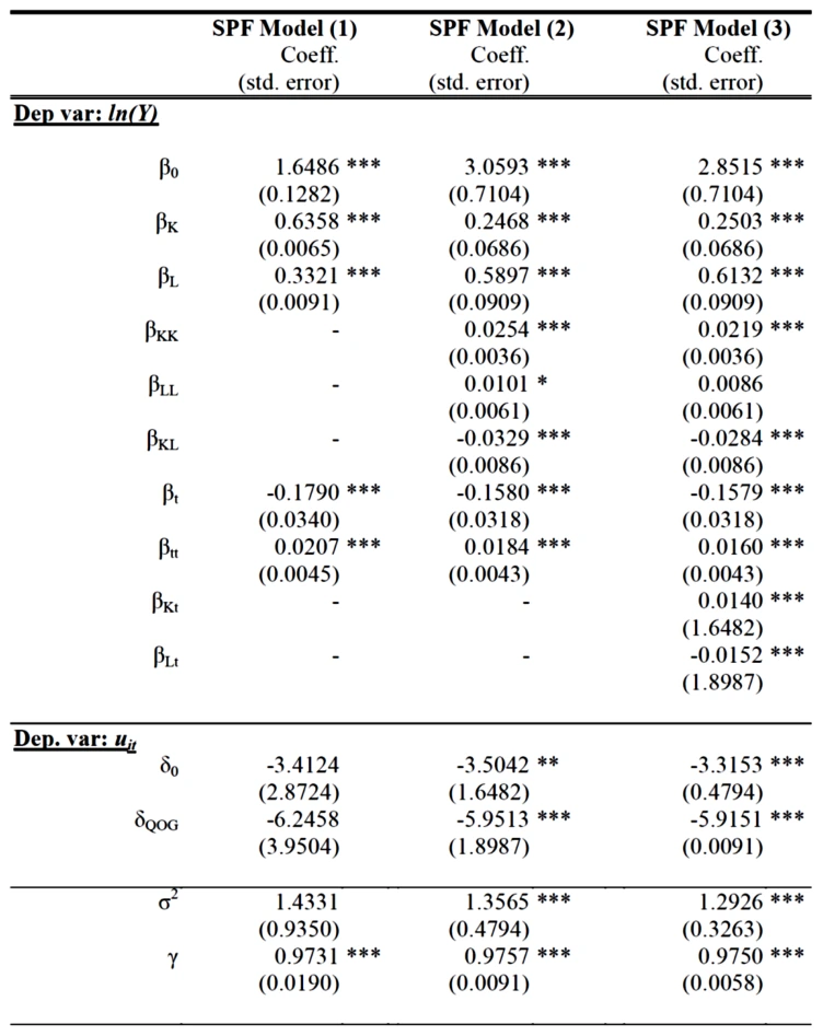
We first take a preliminary test of the specification of the production function as set out in eq. (25). For simplicity, we incorporate QOG, a composite index of the quality of government, as the only explanatory variable in the technical inefficiency model at this stage. The key aim of the results is to provide support to our specification of the production function. Test results are given in Table 2.
A Cobb-Douglas production function is specified in SPF Model (1), A Hicks-neutral translog production function is used for SPF Model (2) and a non-neutral translog production function is in SPF Model (3). As we explained earlier, the translog production function is a more flexible form of the Cobb-Douglas production function. Comparing SPF Models (2) and (3), the former model only accounts for Hicks-neutral technical change. That is, the production function shifts up and down but their slopes (e.g. marginal rate of technical substitution) do not alter. In SPF Model (3), non-neutral technical change is also accounted for by including terms involving the interactions of the other regressors and time. Non-neutral technical change is also referred to as biased technical change. That said, the movement of the production function will be biased in favour of certain inputs and against others.
All three SPF models show that the signs of elasticities of both capital and labour (𝛽𝐾 𝑎𝑛𝑑 𝛽𝐿) are positive as the theory predicted. Compared to the standard assumption of input shares of capital and labour to be one-third and two-third respectively, the parameters in SPF Model (1) show rather awkward results – 𝛽𝐾 is around 0.6 whereas 𝛽𝐿 is around 0.3. In SPF Models (2) and (3), the input elasticities are more sensible. The production functions in both models exhibit a decreasing return to scale, with 𝛽𝐾 is around 0.25 and 𝛽𝐿 is around 0.6.
***, ** and * denote 1%, 5% and 10% statistical significance respectively
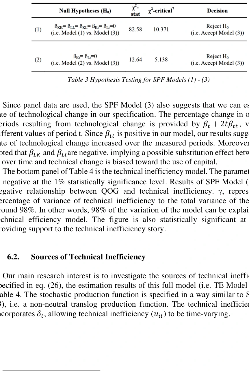
We use the LR-test described in Section 4.2 as a basis for model selection. The test results are summarised in Table 3.7 The hypothesis test suggests that SPF Model (3) is supported. It will also form the baseline specification of our models.
6.2. Sources of Technical Inefficiency
7 Critical values of test statistics are obtained from Kodde and Palm (1986).
***, ** and * denote 1%, 5% and 10% statistical significance respectively
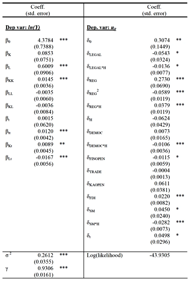
First of all, on the effect of human capital (H) on technical inefficiency, the estimated parameter ( 𝛽𝐻) suggests negative association between the two. This implies that economies with more human capital tend to be more technically efficient, but the effect is not statistically significant.
In terms of institutions, the full model tests their direct impact on technical inefficiency as well as the interactive term of institutions with human capital, which attempts to measure the impact of institutions given a necessary level of human capital. Marketcreating institution, LEGAL and its interactive term with H are both negative and statistically significant, albeit at 10% level only. In other words, economies with better secured property rights and legal system are less technically inefficient. 𝛿𝐿𝐸𝐺𝐴𝐿∗𝐻 is negative, signifying economies with more human capital are less technically inefficient even if their market-creating institutions are comparable.
Such a negative relationship is also found to be statistically significant for parameters of 𝛿𝑆𝑀∗𝐻 and 𝛿𝐷𝐸𝑀𝑂𝐶∗𝐻. However, the direct impact of the market-stabilising institution, SM, and the market-legitimising institution, DEMOC, are found to be positive, although the former is only at 10% significance level and the latter is not statistically significant. These results are not in line with our hypothesis – better institutions tend to reduce technical inefficiency. This prompts us to test the validity of these parameters in the model.
On the impact of market-regulating institution – REG, the results are less straightforward. 𝛿𝑅𝐸𝐺 is positive, suggesting that less regulation is more technically inefficient. It may first appear to be odd. However, this may also imply that there is a potential optimal level of regulation. As we argue earlier, market-regulating institution could be either market-promoting by rectifying monopoly and promoting competition or market-hampering by generating red-tape and bureaucratic delay. In this light, we incorporate a square term REG2 to capture such an effect, which is statistically significant at 1% level. Taking both parameters together, our results suggest a U-shape relationship between technical inefficiency and the level of regulation. It implies that when the economy has a too low level of regulations, introducing more regulations can improve technical inefficiency. However, once the level of regulation reaches a critical point, more regulation will lead to worsening technical inefficiency.
For openness parameters, trade openness and capital account openness (𝛿𝑇𝑅𝐴𝐷𝐸 𝑎𝑛𝑑 𝛿𝐾𝐴𝑂𝑃𝐸𝑁) do not have statistically significant impact on 𝑢𝑖𝑡. Financial openness has a positive impact on improving technical efficiency, although it is only statistically significant at 10% level. Unexpectedly, more FDI inflows associate with technical inefficiency. This is contrary to our expectation that more foreign capital leads to more foreign competition and more efficient use of production inputs. Our results, however, suggest that foreign firms (in the form of FDI) could possibly be more competitive and thus dominate the domestic markets. It thus crowds out the competition from domestic firms.
Against the estimation results of unexpected signs of some parameters obtained in TE Model (1), we deploy the formal LR-Test to test the validity of the coefficients more robustly. The test results are presented in Table 5 below.
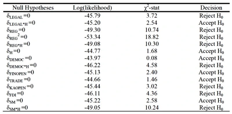
Note: The critical value of the log likelihood ratio test for degree of 1 is 2.706
Table 5 points out that the LR-test rejects the validity and significance of some parameters in our full model – TE Model (1). This facilitates us to re-specify TE Model (1) into TE Model (2). In the latter model, we drop all parameters that can be accepted as zero in the LR-test. The estimation results of TE Model (2) are in Table 6.
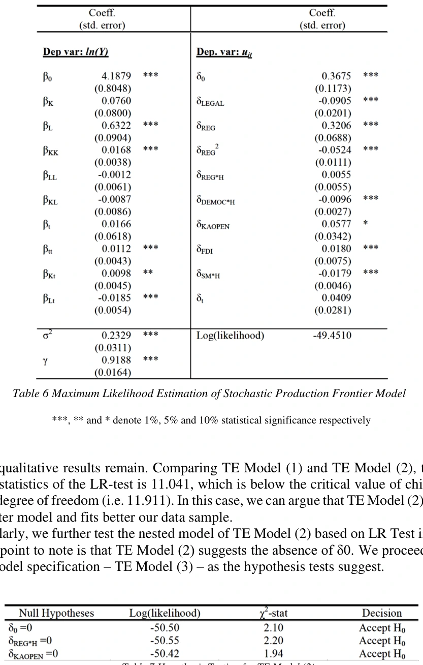

Note: The critical value of the log likelihood ratio test for degree of 1 is 2.706.
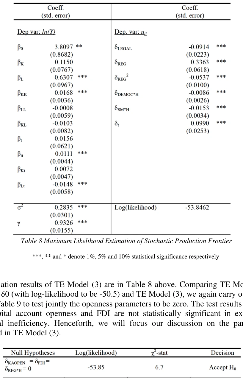

In the course of model selection through TE Models (1) to (3), generally speaking, only institutional factors survive in the final models. Other competing factors – human capital and openness – are not statistically significant in explaining the sources of cross-country technical inefficiencies. This provides empirical support to North’s hypothesis – i.e. institutions are the determinant of the efficiency of production inputs, via which determine cross-country efficiency and hence economic performances. Although there are previous studies which conclude that human capital and openness in trade, foreign capital, capital account or financial integration may promote growth, we do not find such positive effects on technical efficiency. In other words, we argue that the level of technical efficiency is primarily driven by domestic market-friendly institutions rather than external forces like foreign competition brought forward by international trade or capital flow alike.
However, our final model – TE Model (3) – points out that not all clusters of institutions are directly associating with technical inefficiency. Market-creating institution, i.e. the security of property rights (LEGAL) and market-regulating institution (REG and REG2) are directly associating with technical inefficiency. We obtain the negative relationship between these clusters of institutions and technical inefficiency as expected. Marketstabilising institution, i.e. sound monetary policy (SM), and market-legitimising institution, i.e. democratic institution (DEMOC), nonetheless have no direct and significant impact on technical inefficiency. Their interactions with human capital (H) are significantly negative at the 1% level. These results may suggest that these two clusters of institutions would only improve technical efficiency given that a necessary level of human capital. That said, a democratic economy is more efficient given a minimum level of human capital is reached. Likewise, the effectiveness of stabilising monetary policy to improve efficiency of production inputs also depends on human capital. These effects are believed to be determined by human capital, which are possibly due to the effectiveness of policy execution and governance. These market-friendly institutions in turn are believed to shape the incentive structures of the society and thus affect the efficiency of production inputs.
To sum up, our final model suggests that our dataset supports a technical inefficiency story (where γ is statistically significant at 1% level) when estimating a non-neutral translog stochastic production function. The time-varying technical inefficiency model tests three sets of explanatory factors of technical inefficiency – human capital, institutions and openness. Based on the test results of log-likelihood ratio tests, we find no direct effect of openness and human capital on technical inefficiency. However, human capital works with democracy and monetary stabilisation policy to improve technical inefficiency across countries. In contrast, better security of property rights and less regulatory environment associate with technical efficiency directly.
6.3. Measures of Technical Efficiency
Following Coelli et al. (1998), since the SPF model can be defined as
, the measures of technical efficiency are essentially obtained from
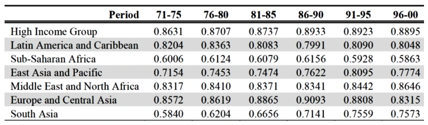
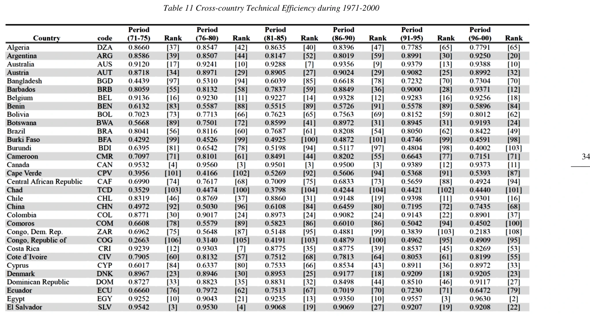
. Technical efficiency (TE) can thus be calculated for each period and compared to the best practice. TE represents the mean value of technical efficiency given the amount of inputs. Since the production function is assumed to be stochastic in nature, the best possible TE lies somewhere below 1 due to stochastic disturbances. A summary table of average TE over the studied period is in Table 10. The complete measure of TE for each cross-section and time period is presented in Table 11.
Over the six measured periods, the USA topped the ranks of TE during 1971-75, 1976-80, 1986-90, and 1991-95. Trinidad and Tobago came first during 1981-85, possibly reflecting it as an oil-exporting economy. Ireland became the best practice in the last measured period, i.e. 1996-2000. The mean TE of the sample is quite stable (around 0.74-0.75) over the three decades. As one can expect, the industrialised economies are among the best practices. In contrast, the least technically efficient economies are mostly Sub-Saharan African countries.
Note: Average TE is calculated based on simple averages. High income group includes OECD economies and other
high income groups. Regions are based on World Bank’s Country Classification.
Details of country coverage are at Appendix A.2.
Analysed by regions, there is a general upward trend of improvement in TE over the last three decades. Improvements are also found in the high income group even though they are amongst the best practices. However, sub-Saharan African countries indeed experienced a decline over the period. The most pronounced improvements are found in the East Asia and Pacific as well as South Asia regions, in particular starting from the 1990. Such improvements are also found in fast-growing countries like China and India during the same period.
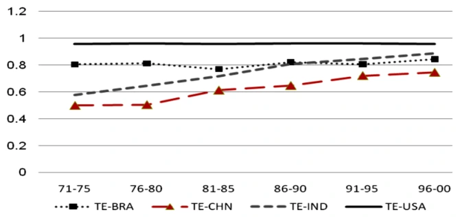
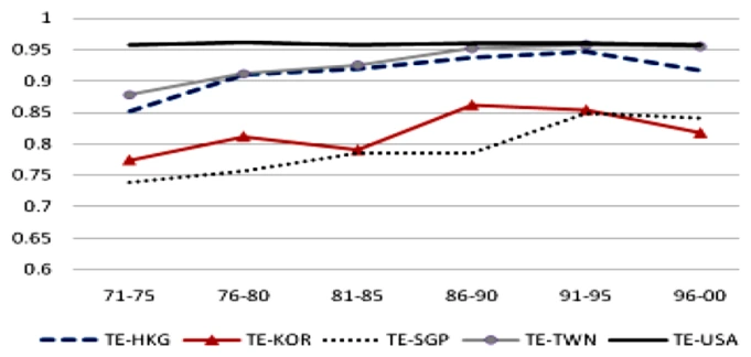
Our measured period is long enough to compare the experiences of economic development in different regions. Figure 1 clearly shows that China and India rapidly caught up with the USA. The catching-up was fairly persistent for India during the studied period. China only started picking up since the early 80s, echoing her “open-door” policy. In comparison to other emerging markets like Brazil, her TE improvements were relatively gentle. We can also compare these growth experiences with that of the “East Asian Tigers” as shown in Figure 2. The latter four economies also enjoyed fast growth during the last three decades. In conjunction, they showed rapid improvements in technical efficiency in the 70s and 80s.
To calculate efficiency change (EC) over two periods, we can define EC as:

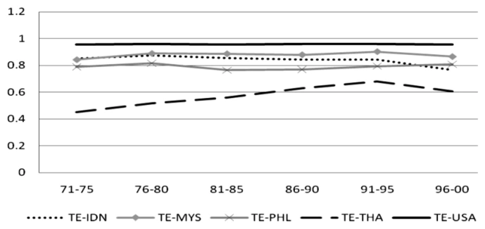
Based on EC calculated, the four “Asian tigers” – Hong Kong, Singapore, South Korea and Taiwan – enjoyed an average efficiency gains of 1.5%, 2.7%, 1.2% and 1.7% respectively over the studied period. These figures represent above-average performances (around 0.85% for the full sample) on the global scale. This may be one underlying source of their impressive growth performances. Nevertheless, India and China show even more impressive improvements. China registered an average 8.6% efficiency change whereas India showed an even more impressive 9.1% positive change. All these provide quantitative evidence that the rapid growth we found in these economies may not be a mere result of capital accumulation. Efficiency improvements may be their sources of growth. Figure 3-Figure 5 provide an overview of efficiency changes in other selected countries.
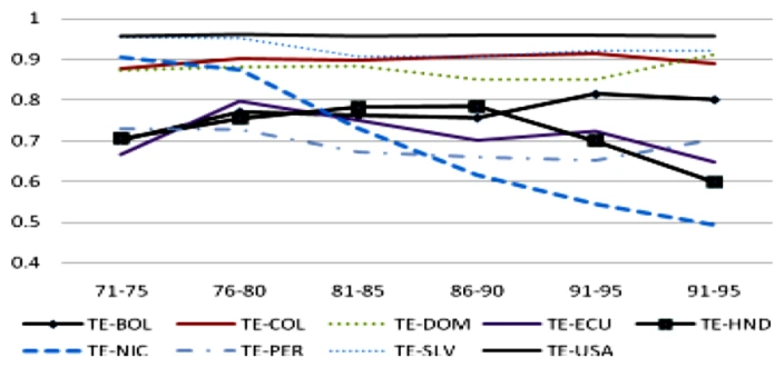
Note: Countries include Bolivia, Colombia, Dominican Republic, Ecuador, Honduras, Nicaragua, Peru and El
Salvador.
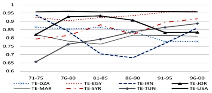
Note: Countries cover Algeria, Egypt, Iran, Jordan, Morocco, Syrian Arab Republic and Tunisia.
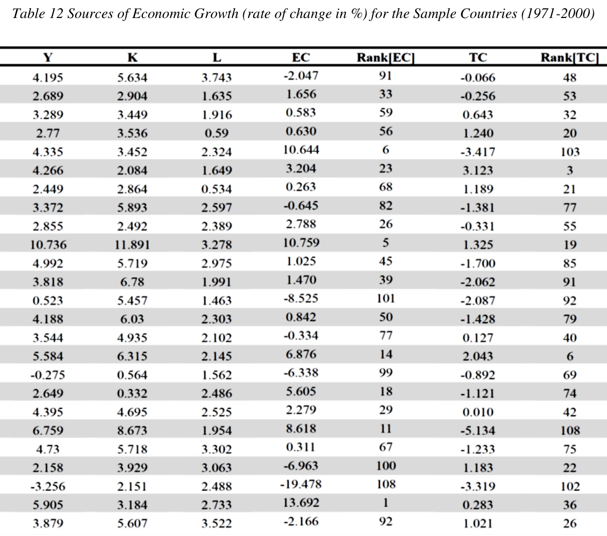
To better illustrate that efficiency change is possibly the source of growth, we separate the sources of growth by capital accumulation, technical change and efficiency change. As mentioned earlier in our methodology, estimating a time-varying stochastic production frontier allows us to estimate technical change (TC) and TE. Technical change is calculated based on the first partial derivative of the stochastic production frontier with respect to time. According to Coelli et al. (1998), a geometric mean can be used to estimate the technical change index between adjacent period’s s and t as the following:
![0.5 [ {1 + 𝜕𝑓(𝑥𝑖𝑠 , 𝑠 , 𝛽) 𝜕𝑠 } × {1 + 𝜕𝑓(𝑥𝑖𝑡 , 𝑡 , 𝛽) 𝜕𝑡 } ]](/static/article-media/cross-countries-economic-performances-spf-approach/equation-051.png)
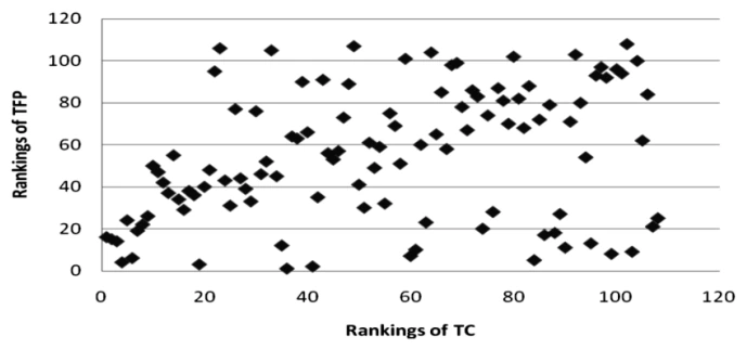
Once we have decomposed growth, it also facilitates us to compare the sources of growth in developed countries as against that in developing countries. Rankings of efficiency change reveal that the sources of growth in developing countries primarily come from efficiency gains. Most of the economies topping the rankings of efficiency changes (i.e. with greatest efficiency gains in the sample) are low or lower middle income countries – for examples, Republic of Congo, Pakistan, Botswana, Bangladesh, India and China. In contrast, the sources of growth for high-income or developed countries come from technical changes (i.e. technological progress). For example, in terms of technical changes, Luxembourg, Iceland, Singapore, Norway and New Zealand are amongst those showing most distinct technical changes. This points out that the development strategy for developing countries mainly aims at “catching-up”, whereas that of the developed countries is by means of innovations.
Since our sample is dominated by developing countries, we naturally find a strong correlation of TFP and EC. For demonstration purpose, Figure 6 shows a simple correlation plot between the rankings of TFP as against that of EC and TC of the 108 economies being studied in our sample.
The most important lesson of decomposing the sources of growth after all is not the comparison of rankings. The main point to note is that when we compare cross-country TFP growth using a standard Solow-growth accounting framework (i.e. by assuming that all factors of production are efficiently used), the results obtained may only reveal a partial picture of the sources of growth. Through estimating a stochastic production frontier, we are able to segregate the two sources conceptually. More importantly, we could identify the sources of technical inefficiency which is helpful in implying policy implications.
7. Concluding Remarks
In this paper, we point out that conventional growth empirics are not sufficient to understand diverse economic performances. Measuring technical efficiency may be more in line with the theoretical foundation of explaining cross-country economic performances. Compared to TFP measurement, using an SPF approach may help us understand the sources of growth better as this methodology also allows us to disentangle technical change and technical efficiency change. In addition, the model allows us to incorporate explanatory factors of technical inefficiency.
In terms of investigating the sources of technical efficiency, we identify three key competing views on potential sources, firstly human capital, secondly openness and last but not least institutions. In the existing literature, there is no conclusive empirical evidence showing which factors are more prominent. Effects of these deep determinants also depend on the level of economic development.
We apply the Battese & Coelli (1993) model to estimate technical efficiency and incorporate its determining factors in a single model. Using a translog stochastic production function specification, we cannot find empirical evidence to show that human capital, trade openness, financial integration and capital account openness have direct impacts on explaining cross-country technical inefficiency. In terms of institution, we find that the rule of law has a direct impact on decreasing technical inefficiency. Regulation, nevertheless, shows an optimal level. That said, only after reaching a threshold of a minimum amount of regulation, does too much regulation leads to technical inefficiency. Democracy and stability of monetary policy have no direct impact on technical inefficiency as our empirical results show. However, their interactions with human capital in turn are statistically significant. It implies that these two aspects of institutions only work with a given level of human capital to improve technical efficiency. Our findings seem to support the view of North and Parente and Prescott’s theory that to reduce the income gap between developed economies and developing economies, the late starters have to use resources by making improvements in their institutional quality.
Our model also shows that technical efficiency is time-varying. Based on our estimated stochastic production frontier, we can proceed with deriving cross-country efficiency changes and technical changes. As expected, the industrialised economies are among the best-practice. Comparing the performances across regions, we find that emerging markets like China and India experienced drastic improvements in technical efficiency. Sub-Saharan African countries stayed well below the frontier over our studied period, although the performances of individual countries are quite diverse. When we further segregate the sources of growth into efficiency changes and technical changes, we find that the main source of growth in developing countries is through the channel of efficiency change. In developed economies, in contrast, the source of growth primarily comes from technical change (i.e. technological progress).
Our research helps our understanding of the economic importance of institutions. Also, it attempts to quantify to what extent market-sustaining institutions could hamper economic performances. Our quantifiable indicator is the estimated mean level of technical efficiency, as compared to that of the best practice. One of our major findings is that income disparities across countries may result from the way production inputs are allocated, rather than factor accumulation.
This study provides empirical support to demonstrate what the likely and potential benefits of structural reform are that help strengthen market-sustaining institutions. In particular for developing countries, as we find, the main source of growth comes from efficiency change, which in turn relies on institutions and their interaction with human capital.
Limitations
Data limitation is also a major problem. On one hand, all the institutional variables are measuring the macroeconomic environment, without specific reference to particular sectors or industries. Variables with a particular focus at the micro-level may help strengthen further how development outcomes interact with the institutional arrangement. On the other hand, we only have three decades of institutional variables so far. Over time, when more data come up from different sources, more studies on institutional change can be undertaken for checking robustness and sensitivity.
About the Research
A series of five papers contrived from my MPhil thesis entitled "Essay on Institutions, Policies, and Economic Development" was constructed of six chapters at University College London (UCL). The first paper is an overview, and the other four papers are empirical studies looking at the effects of institutions on economic growth across the country. The first paper, entitled "Institutions, Policies, and Economic Growth Overview", reviews the relationship between institutions and policy regulation with development from the perspective of economic literature. The second paper, entitled “Impact of Institutions and Policy on Economic Growth: Empirical Evidence", empirical analysis to explore the interaction between the institution and economic growth. The third paper, entitled “Role of Political Institutions on Economic Growth: Empirical Evidence”, is an empirical analysis to explore the effect of political institutions on development. The fourth paper, entitled “Impact of Natural Environment, Regional Integration, and Policies on FDI”, explores the effects of three determinants of bilateral FDI, including natural barriers, the “at-the-border” barrier (regional trade agreement), and the “behind-the-border” barrier (domestic regulatory environment). The fifth paper, entitled “Cross Countries Economic Performances -SPF Approach”, explores the differences in technical inefficiency (inefficient allocation of production inputs) and explains the diverse cross-country economic performances, using estimating a “global” stochastic production frontier (SPF) mod.
Acknowledge
I would like to express my sincere gratitude to my supervisor Professor Orazio Attanasio, who has been very resourceful in supporting and guiding me throughout my MSc study. Also my deepest thanks to Professor Sir Richard Blundell, for his valuable suggestions, comments, and guidance.
APPENDICES
A.1 Descriptive Statistics and Correlation Matrices
Descriptive Statistics of Institutional Variables
Correlation Matrix of Institutional Variables
A.2 List of Economies
List of Panel Units - Country Coverage
Note: Country code and income group classifications are based on World Bank Country Classification.