Impact of Natural Environment, Regional Integration, and Policies on FDI

1. Introduction

The extension of the international market in the form of foreign direct investment (FDI) is one of the most salient features of globalisation since 1980. For both developing and developed economies, FDI is an important source of capital, technology and skills transfer. FDI outflow on the other hand helps the source economy to enjoy market expansion, lower factor costs and facilitate “tariff-hopping”. All these suggest that FDI could potentially lead to economic growth and economic development.

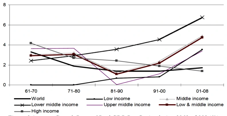
FDI indeed experienced a distinct upsurge in the last few decades, alongside accelerating growth worldwide (see Figure 1). Figure 2 shows that total FDI inflows¹ only amounted to some US$54 billion in 1980, subsequently increasing to US$1,833 billion in 2007. This represents an impressive average growth rate of almost 14% per annum. Although it fell dramatically to US$561 billion in 2003 due to the IT bubble burst, it rose significantly again in 2007 and reached a new peak.

¹ According to UNCTAD’s definition, FDI inflows and outflows comprise capital provided (either directly or through other related enterprises) by a foreign direct investor to an FDI enterprise, or capital received by a foreign direct investment from an FDI enterprise. FDI includes the three following components: equity capital (foreign direct investor's purchase of shares of an enterprise in a country other than that of its residence), reinvested earnings (direct investor's share (in proportion to direct equity participation) of earnings not distributed as dividends by affiliates or earnings not remitted to the direct investor. Such retained profits by affiliates are reinvested) and intra-company loans (referring to short- or long-term borrowing and lending of funds between direct investors (parent enterprises) and affiliate enterprises).

FDI stock refers to the following. For associate and subsidiary enterprises, it is the value of the share of their capital and reserves (including retained profits) attributable to the parent enterprise (this is equal to total assets minus total liabilities), plus the net indebtedness of the associate or subsidiary to the parent firm. For branches, it is the value of fixed assets and the value of current assets and investments, excluding amounts due from the parent, and fewer liabilities to third parties: http://www.unctad.org/Templates/Page.asp?intItemID=3201&lang=1.

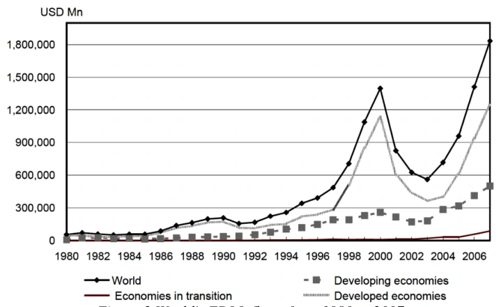
Albeit such a distinct surge, we consistently find that the significant share of foreign capital only flows between developed economies. Analysed by regions in Figure 3, FDI inflows to the developed economies alone accounted for the largest share of some 55-86% of the world’s total during the period 1980-2007. The corresponding shares of the developing economies and transitional economies did pick up, yet remain far behind in overall terms.

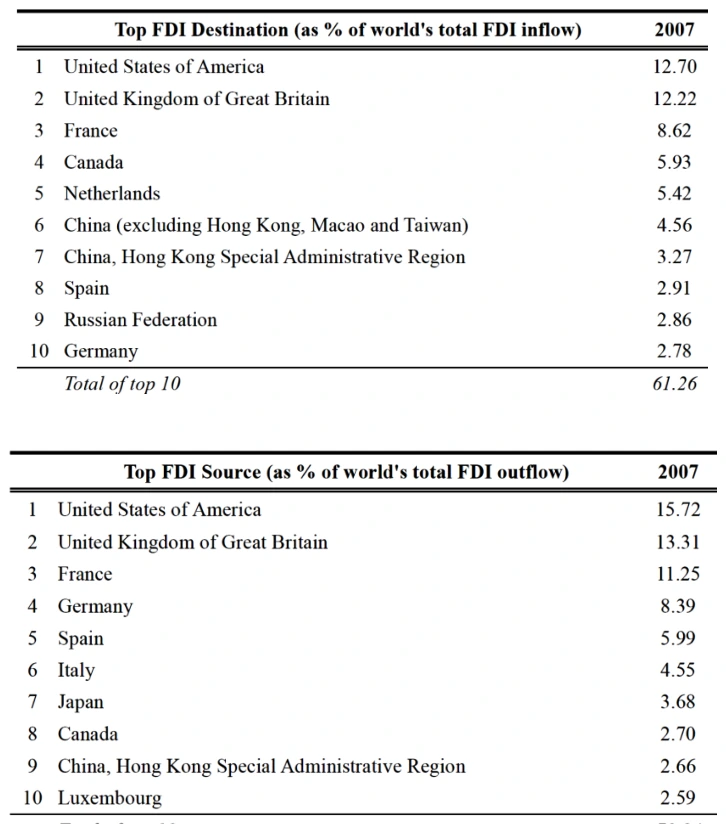
Not only are the major FDI destinations, but developed economies are also the major FDI sources. Table 1 shows that the top 10 FDI destinations and sources in 2007 are mostly OECD economies, except for the case of China and Hong Kong. The latter is due to the fact that a significant share of Hong Kong’s FDI came from Mainland China, accounting for about 25% (2007 figure) of China’s total FDI outflows. OECD economies as a whole accounted for 85% of the world’s FDI outflows and 84% of FDI outward stock in 2007.

Typeset table reconstructed from version-of-record PDF page 4. Select the image to open the full-resolution facsimile.

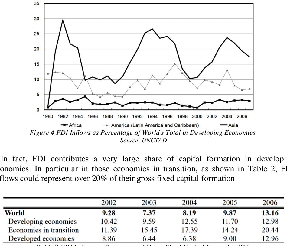
In terms of FDI inflow in developing countries (see Figure 4), Asia and Latin America countries accounted for the greatest shares of the world’s total FDI inflows of some 17.4% and 6.9% respectively in 2007. Whilst Africa is the poorest region, its respective share has been consistently less than 5% for the last few decades.

Typeset table reconstructed from version-of-record PDF page 5. Select the image to open the full-resolution facsimile.

As FDI is one of the major sources of capital accumulation and can act as a vehicle of technological progress through the use and dissemination of improved production techniques, attracting FDI therefore naturally forms part of the growth strategy of most developing economies. However, we are left wondering why capital does not flow from the rich economies to the poor, where production costs are low and marginal productivity of capital is high.

In this light, the literature has been extensively developed to study the determinants of FDI. Studies at the micro-level suggest that the structure of the industry, factor cost of production and intra-industry scale effect, amongst others, may affect investors’ decisions to invest abroad in the form of greenfield FDI or mergers or acquisitions. Another strand of the literature investigates the macroeconomic determinants. It essentially argues that specific characteristics of the destination economy play a significant role, such as the transportation cost between the destination economy and source economy, trade barriers, fiscal incentives, business climate and exchange rates etc. This study belongs to the latter strand, i.e. identifying the determinants of FDI at the macro level.

Our key research objective of this paper is to assess three potential macroeconomic determinants of FDI, namely, a natural barrier, de jure “at-the-border” external institution and de facto “behind-the-border” domestic institution. This is motivated by the fact that regional integration and behind-the-border regulatory obstacles have lately drawn the keen interests of policymakers intending to improve institutional frameworks, regulatory environment and government policies for attracting foreign investment. We intend to evaluate their respective impacts under a unified assessment framework.

Following the existing literature on trade and capital flow, we refer to natural barriers as the geographical characteristics and historical ties between the destination and source economies. We expect that geographical and cultural proximities reduce transportation and transaction costs, thereby fostering bilateral FDI flows.

In the “behind-the-border” domestic institutional environment, recent research has focused on the rule of law, development of the credit market, political stability and business and investment climate etc. Our specific focus here is to investigate how the regulatory environment of the destination economy affects FDI. It is believed that holding other factors constant, a burdensome regulatory environment discourages foreign investors to invest due to the enormous costs of compliance and association corruption (see Wei (2000b)), thereby hampering the dynamics of firm entry and the degree of local competition. On the contrary, a less regulated environment reduces the sunk costs to invest offshore for foreign investors and is thus more likely to attract FDI.

“At-the-border” external institution refers to regional integration, reflected by bilateral (or regional) trade agreements (henceforth RTAs). Although most RTAs aim at facilitating trade liberalisation, positive impacts on FDI are also possible. This is because closer integration is also likely to associate with an expansion of the total market size.

We intentionally test de jure “at-the border” external institutions (i.e. RTAs) and de facto “behind-the-border” domestic institutions together. We consider the former as an externally imposed institution, while the latter is a de facto institution in the sense that the variable we used measures the subjective perception of the regulatory environment. The scores are collected from foreign investors in the respective economies. This score to a certain extent, albeit imperfectly, reflects the domestic regulatory environment. Our investigation hence may allow us to understand which type of barriers, natural or institutional, determines the relative locational advantages of FDI.

Our work in the following is entirely empirical and uses an augmented gravity model for our estimations. We hypothesise that a better domestic regulatory environment may lead to more FDI inflows. Reciprocally, more FDI inflows may also lead to a better regulatory environment since the domestic government may respond to the needs of foreign investors. Such endogeneity will be taken into account in our study. Unlike the existing literature, which focuses on the impacts of the overall institutional environment and regional agreements on aggregate FDI inflows,² we use bilateral FDI data instead of aggregate FDI data. As we discussed earlier, OECD economies are the key FDI destinations and sources.

² Nevertheless, it is not our intention to assess the impact of each regional trade agreement on FDI, nor the effectiveness of each agreement. Studies have been done to assess the impact of the individual regional trade agreement on bilateral trade, especially the effect of WTO accession.

Our dataset will thus focus on bilateral FDI data of OECD economies as sources. Using bilateral FDI data at the same time could also improve the accuracy of our estimations. It is because aside from the variables of our interest, there may also be some characteristics that are specific to the destination and source economies. Hence, to minimise omitted variable bias, we can control for the specific country-pair heterogeneity when using bilateral data, which cannot be achieved using aggregate FDI data.

This paper is probably among the very first few to assess the impact of natural barriers, regional integration and regulatory environment altogether on bilateral FDI. The results may help develop policy implications by identifying the macroeconomic determinants of FDI.

The rest of the paper is organised as follows. Section 2 provides a brief literature survey. We describe the data used in Section 3. In Section 4, we discuss the estimation strategies. Empirical results are presented in Section 5. We conclude and set out the policy implications in Section 6.

2. Literature Survey: Regional Integration and Regulations as FDI Determinants

The first generation of literature on FDI was largely devoted to its macroeconomic impacts. It is argued that FDI promotes economic growth and development since FDI provides a new source of capital, thereby allowing investment in both human and physical capital on one hand. On the other hand, it also serves as a means to incorporate new knowledge and technology from abroad. Amongst others, Borensztein, De Gregorio, and Lee (1998) use data on FDI flows from industrial countries to 69 developing countries from 1970 to 1989 and suggest that FDI is an important vehicle for the transfer of technology, contributing relatively more to growth than domestic investment does. Empirical results from Balasubramanyam, Salisu and Sapsford (1996) on the other hand suggest that FDI may be growth-promoting only in export-promoting countries rather than in import-substituting ones. More recently, Li and Liu (2005) use data from 84 countries from 1970 to 1999. Both single equation and 3SLS estimations show that there is a robust positive relationship between FDI and economic growth.

The second generation of literature focuses more on the determinants of FDI and investigates the underlying factors of the locations of foreign affiliates. In particular, the quality of institutions increasingly plays a pivotal role in attracting foreign investment since good governance is usually associated with better security of property rights, an effective legal system and enforcement of regulations, a well-built physical and financial infrastructure and a generally more productive environment.

³ See Subramanian and Wei (2007) and Eicher & Henn (2009).

In his survey, Lim (2001) succinctly summarised seven key macroeconomic aspects of FDI determinants. Four of them are particularly relevant to our work. They include (1) economic distance/transport costs; (2) size of the destination market; (3) business/investment climate and (4) trade barriers/openness.⁴ Their net impact, however, depends on the nature of FDI – vertical or horizontal FDI.

2.1. FDI and Natural Barriers

Lim (2001) argues that the impact of economic distance (and hence transport costs) on FDI is conceptually unclear. Horizontal FDI (i.e. “market-seeking” FDI) will tend to replace exports and thus increase if the cost of market access through exports is high or if the distance between the source and destination markets is large. Nevertheless, as vertical FDI (i.e. “production cost-minimising” FDI) is generally export-oriented, it may then be discouraged by high transport costs.

Similarly, for market size – measured in terms of economic activity, population or area, a larger destination market will encourage horizontal FDI as it will reduce the cost of supplying that market as a result of economies of scale and lower unit fixed cost. Vertical FDI, on the other hand, may be indifferent to this factor.

In overall terms, there is no conclusive argument about the combined effect of economic distance and market size on FDI inflows. Along this line, our estimations will capture the effect of natural barriers on FDI and empirically test these two effects.

2.2. FDI and Regulations

Lim (2001) further identifies that the lower costs of doing business in a foreign country, holding other factors constant, are more attractive to FDI. These costs may include regulatory, bureaucratic, and judicial hurdles, issues of property rights, the enforceability of contracts, labour regulation, and political and macroeconomic stability.

The literature relating the institutional quality of the destination economy as the determinant of FDI often relies on the use of an aggregate index of institutions. The choice of “institutional” variables is also different in different studies. Wheeler and Mody (1992) are amongst the first to investigate the impact of the institution on FDI. They use a composite index of risk factors, which include bureaucratic red tape, political instability, corruption and quality of the legal system, and show that there is no significant impact of institutions on determining the location of US foreign affiliates. Singh and Jun (1995), in contrast, show that a general qualitative index of business operation conditions is an important determinant of FDI in countries that receive high flows. In addition, they also find that these countries also show a positive relationship between taxes on international transactions and FDI flows – i.e. supporting the “tariff jumping” hypothesis.

⁴ Another three factors include agglomeration effects, factor costs and fiscal incentives, which are not the factors of our direct interest in this paper. Recent research studies additionally emphasize the effect of exchange rate on FDI flows (see Froot and Stein (1991), Blonigen (1997) and Blonigen (2005)).

Wei (2000a) focuses on one specific aspect of an institution – corruption. He finds that corruption and so as the uncertainty of corruption have significant negative effects on FDI. Likewise, Stein and Daude (2002) show that inward FDI is significantly influenced by the quality of institutional variables. Political instability and violence, government effectiveness, regulatory burden, rule of law and graft all matter for FDI. Political institutions, e.g. political representation and accountability indicators, on the other hand, do not.

By studying the effects of institutions on capital structure, Aizenman and Spiegel (2004) find that the ratio of FDI to gross fixed investment, as well as the ratio of FDI to private domestic investment, is negatively and significantly correlated with the level of corruption. This suggests that FDI is more sensitive than domestic investment to the level of institutional quality. By using the law and order variable of ICRG instead of corruption, Albuquerque (2003) likewise finds a negative yet insignificant effect.

More specifically regulation and its impacts on various economic outcomes are extensively studied.⁵ Its role in attracting FDI is less frequently explored. Regulations are generally justified as a way for governments to serve the public interest and address externalities or market failures. Indeed, there are legitimate and important functions fulfilled by regulations. However, regulations can also carry costs in terms of bureaucratic delays or expenses to meet compliance that too often has little bearing on the rationale of the regulation. Particularly in developing countries, excessive regulations usually lead to widespread corruption.

Only recently, there are a few papers specifically devoted to regulation and FDI. Hermes & Lensink (2003) and Alfaro, Chanda, Kalemli-Ozcan, et al. (2004) examine the linkages between financial market regulations, FDI and growth. They both concur that countries with better financial systems and financial market regulations can exploit FDI more effectively and thus achieve high growth rates. A well-functioning financial market allows entrepreneurs to obtain credit for their new businesses or business expansion. As such, countries could benefit from inward investment to promote economic growth.

Busse and Groizard (2006), on the other hand, study the impact of broader government regulations on the interaction between FDI and growth. They argue that countries need a sound business environment in the form of good government regulations to be able to benefit from FDI. Countries may only benefit from foreign investment flows if they have appropriate local government regulations and institutions in place. Excessive regulations are likely to restrict growth through FDI if human and capital resources are prevented from reallocation. Using the World Bank’s Ease of Doing Business Indicators, they find evidence that excessive regulations restrict growth through FDI only in the most regulated economies. This result holds for both OLS and 2SLS estimations. Their findings also suggest that FDI does not stimulate growth in economies with excessive business and labour regulations, after controlling for GDP growth rates.

⁵ For example, a number of papers find important effects of labour regulations on firm entry, job creation and economic growth (e.g. Botero, Djankov, Porta, et al. (2003), Besley and Burgess (2004), Almeida and P. (2005), Haltiwanger, Scarpetta, and Schweiger (2006), Petrin and Sivadasan (2006) and Autor, Kerr, and Kugler (2007)). Other papers examine the effect of business regulations on firm entry, growth and informality (see Djankov, Porta, Lopez-de-Silane, et al. (2003b) and Loayza, Oviedo, and Servén (2004)). Others look at regulatory developments in the financial market (e.g. Beck, Demirguc-Kunt, and Maksimovic (2005), Demirguc-Kunt and Maksimovic (1998), Galindo and Micco (2005)). Almost all of them focus on cross-country variations.

Our work follows the line of Busse and Groizard (2006) to examine the impact of government regulations on FDI. However, our approach has a number of differences. Firstly, we use various sub-indices from the Fraser Institute’s Economic Freedom Index to measure government regulations. Like the World Bank’s survey, our indicators are also subjective in nature. However, our time span covered is longer, which allows us to undertake panel data analysis. Therefore, unlike Busse and Groizard (2006), which is cross-sectional in nature, our models introduce a greater degree of freedom. As their analysis is cross-sectional, they have to rely on clustering samples or incorporating regional dummies to capture the specific heterogeneity of the destination economies partially. In our case, panel data models readily allow us to capture the unobserved panelspecific heterogeneity. Finally, like other empirical work studying the impact of institutions on FDI, aggregate FDI data are often used. One limitation as such, as pointed out by Bénassy-Quéré, Coupet, and Mayer (2007), is that the specific characteristics of the destination and source economies cannot be included at the same time since the estimations do not rely on bilateral FDI data. In other words, these empirical studies primarily assessed the impact of the overall institutional environment of the destination economy on FDI inflows.

More recent research henceforth has started to explore the FDI determinants more specifically in respect of characteristics of the destination and source economies. Using bilateral FDI data is therefore inevitable. Table 3 below summarises some recent empirical studies estimating the impact of institutions on bilateral FDI flows/stocks. However, as we note, the majority of these empirical estimations still rely on crosscountry analyses due to the short time span of institution data. Specific analyses on the three determinants as we proposed do not yet exist so far.

Typeset table reconstructed from version-of-record PDF page 11. Select the image to open the full-resolution facsimile.

2.3. FDI and Regional Integration

Regionalism is indeed one of the key features of recent global development. According to the World Trade Organisation (WTO),⁶ RTAs in recent years have become a very prominent feature of the Multilateral Trading System. The surge in the number of RTAs has continued unabated since the early 1990s. Some 421 RTAs have been notified to the GATT/WTO up to December 2008. On that same date, 230 agreements were in force.⁷ RTAs were used to focus on removing trade barriers on goods, but are later expanded to cover trade in services and bilateral investment.

⁶ Source: www.wto.org.

Blomstrom & Kokko (1997) are amongst the first to assess the impact of regional integration on FDI. Focusing on three specific RTAs,⁹ they find that the impacts of a regional agreement on FDI largely depend on the environmental change brought about by the agreement. If the regional agreement leads to improved resource allocation and increased competition, overall economic efficiency is expected to be enhanced as a growth rate. The effects also depend on the locational advantages of the participating countries and industries.

Their empirical findings also suggest that RTAs bring a more positive significant impact on FDI if RTAs coincide with domestic liberalisation and macroeconomic stabilisation in the member economies.

The ambiguous results, as they argue, may also arise from the potentially offsetting influences from two dimensions. On one hand, some FDI continues to be motivated primarily by the desire to get behind trade barriers. Another FDI is motivated by foreign investors seeking to exploit input or output markets located abroad in activities were operating a foreign affiliate is the most efficient governance structure. Nevertheless, a reasonable generalization is that regional integration should enhance the attractiveness of investing in the region as a whole by creating a large common market and contributing to the improved overall efficiency and higher income levels in that market.

⁷ If we take into account RTAs that are in force but have not been notified, those signed but not yet in force, those currently being negotiated, and those in the proposal stage, the figure is close to 400 RTAs which are scheduled to be implemented by 2010. Of these RTAs, free trade agreements (FTAs) and partial scope agreements account for over 90%, while customs unions account for less than 10%.

⁸ Retrieved from http://www.wto.org/english/tratop_e/region_e/regfac_e.htm. ⁹ Their work assessed North-North integration (Canada joining CUSFTA), North-South integration (Mexico’s accession to NAFTA) and South-South integration (MERCOSUR).

To test whether such an expanded market size effect could have resulted from RTAs, Jaumotte (2004) examines a sample of 71 developing countries during the period 1980 to 19999 and concludes that the aggregate market size of the RTA imposed a positive impact on FDI inflows of the member countries. Nevertheless, not all countries in the RTA benefitted to the same extent. In particular, countries with a relatively more educated labour force and/or a relatively more stable financial situation tend to attract a larger share of FDI at the expense of their RTA partners. He also suggests that for all RTA countries, it is essential to improve the business environment. More generally, the creation of an RTA may stimulate virtuous competition between the participating countries, forcing them to improve their investment environment to the best available in the region.

To sum up, the positive effects of RTAs on inward investments can go through two channels. The first-order effect of RTAs is the market size effect. An expanded market size as a result of RTA also encourages both inter-regional and intra-regional vertical FDI. The second-order effect is the result of keener competition amongst member states, leading to greater efficiency and perhaps a better business environment. These, thereafter, may increase interregional FDI as a result of the RTA.

3. Data

3.1. Dependent Variable

The dependent variable we use for the present study is the bilateral outward FDI stock from the OECD International Direct Investment Statistics (Vol. 2008 release 01). As Bénassy-Quéré, et al. (2007) suggest, there are several advantages to working on stocks rather than flows. Firstly, foreign investors decide on the global allocation of output, hence on capital stocks. Second, stocks account for FDI being financed through local capital markets. It is therefore a better measure of capital ownership. Last but not least, stocks are much less volatile than flows which are sometimes skewed by one or two large takeovers, especially in relatively small countries. Implicitly, by using stock figures, we assume that capital can be flowing in and out of the economy instantaneously in response to the determinants we identified.

As we explained earlier, OECD economies account for the largest share of global FDI inflows and outflows. Hence, the aforementioned OECD database covers a significant share of global capital flows. The database covers most of the observations corresponding to FDI sourcing from each of the 30 OECD member economies, to destination economies which are either OECD economies or emerging and developing economies. Our dataset covers 28 OECD source economies (except Belgium and Mexico due to data limitation) and 60 destination economies (30 OECD and 30 non-OECD economies). A full list of economies covered is in Appendix Section A.2. Bilateral FDI stock data covers the period from 1985 – 2006.

A total of 16,183 observations are available. A non-negligible portion of them is zero observations, amounting to 2,169 observations (around 13% of the total). Since we will work on the log-form of FDI data, dropping zero observation may give rise to selection bias. As such, a conventional solution to this problem is to estimate 𝑙𝑛(𝑎+ 𝐹𝐷𝐼) (where a is a constant) instead of estimating ln(FDI). We use a =0.3, and therefore the dependent variable for estimation, labelled as 𝑙𝑛𝑓𝑑𝑖, implies 𝑙𝑛(0.3 + 𝐹𝐷𝐼)⁸ as in Bénassy-Quéré et al. (2007).

3.2. Independent Variables

3.2.1. Gravity Variables

Since we will use an augmented gravity model (to be discussed in detail in the next paper) to estimate the impacts of natural barriers, regional integration and regulatory environment on FDI, the specification will include some standard gravity variables. To capture the market sizes of the source and destination economies (denoted by subscript i and j respectively), we will use three measures. First is the natural log of real GDP (expressed in constant US dollars) (i.e. ln(GDP𝑖) 𝑎𝑛𝑑 ln(GDP𝑗)). Second is the natural log of the population ( ln(POP𝑖) 𝑎𝑛𝑑 ln(POP𝑗), (These data come from the World Development Indicators (WDI)). The third is the log product of land areas of economies i and j (ln(Area𝑖𝑗)) to demonstrate the combined market size impact. Data are from Rose (2004).

Concerning “natural barriers” in the gravity model framework, we incorporate the geographical and historical variables as in Rose (2004)’s specification. These include the natural log of the distance between economy i and j (ln(Dist)), a land border dummy for the pair of economies sharing the same border (Border), a common language dummy (Common Lang), a dummy for the economy-pairs ever in a colonial relationship (Colonyij) Rose (2004), a dummy for having a common colonizer (Common coloniser) and a dummy for the destination economy is an island (Island). These time-in-varying variables are obtained from Rose (2004).

3.2.2. Regional Integration and Regulatory Variables

The “At-the-border” barrier refers to whether the two economies are in an RTA (RTA), a constructed dummy variable to proxy regional integration. Based on Rose (2004)’s database on bilateral RTA membership,¹⁰ we further update the database with respect to the 60 economies of our interest from 2000 onwards. Information is gathered from the WTO’s website. In total, an addition of 20 more RTAs or bilateral trade agreements is augmented in our dataset. Details of this information are in Appendix Section A.1 and A.3.

To measure “behind-the-border” domestic regulatory institutions, we employ subindicators of the Fraser Institute’s Economic Freedom Index from Gwartney, et al. (2008). We use the “catch-all” index of the regulation (REG) as a measure of the overall regulatory environment, ranging from 0 to 10 with a higher score signifying less regulatory burden on the economy. Sub-indices on measuring credit market regulations (Credit Reg), labour regulations (Labour Reg) and business regulations (Business Reg) will also be tested separately. That said, a total of 4 different regulatory variables will be used, ranging from a “catch-all” broadest measure to specific components. Nevertheless, ratings on business regulation are only available since 1995. Hence the sample size is significantly reduced.

The regulatory index intends to measure the regulatory restraints of the credit, labour and product markets. Credit Reg measures the degree of using a private banking system to allocate credit to private parties. Economies that refrain from controlling interest rates receive higher ratings from these components. Labour Reg measures the regulation of the labour market. If wages are largely determined by market forces, hiring and firing conditions are well established and the use of conscription is retrained, the economy will have a higher score. Business Reg identifies the extent to which regulations and bureaucratic procedures restrain entry and reduce competition. Less business regulations result in higher scores.

The composite index of REG is calculated based on quantitative hard data (e.g. percentage of domestic credit consumed by the private sector) where appropriate as well as qualitative business survey data from compiled sources such as the World Economic Forum’s Executive Opinion Survey and World Bank’s Ease of Doing Business (EoDB) Survey.¹¹ The latter data source, as we discussed in our literature survey, is also very prevalently used in the empirical literature since it provides a consistent and comparable methodology for measuring cross-country regulatory environment. We, however, do not directly employ EoDB’s data to measure regulation because the survey only started in 2003. Such a short period imposes many difficulties and limitations to carry out panel data analysis. In contrast, by constructing a composite index on regulation from various sources, the Fraser Institute’s indices span over a reasonably long time. A detailed description of the regulation index and its sub-components is in Appendix Section A.1.

¹⁰ Rose (2004)’s RTAs dataset covers EU, USIS, NAFTA, CARICOM, PATCRA, ANZD, CACM, MERCOSUR, ASEAN and SPARTECA. Only EU, NAFTA and SPARTECA are relevant to the economies covered in our dataset. See Appendix Section A.3 for the full names of these abbreviations.

¹¹ Further information on the Ease of Doing Business Report can be retrieved from, http://www.doingbusiness.org/.

3.2.3. Instrumental Variables

FDI and the regulatory environment could be endogenously determined. More foreign investment may prompt the government to respond closely to the needs of foreign investors by improving the business environment and relieving the excessive regulatory burden of doing business. In return, destination economies, with a better quality regulatory environment, are more appealing to foreign investors and are more likely to attract inward investment. Nevertheless, there is so far neither theoretical nor empirical work suggests any sound and valid instrumental variable which directly affects the domestic regulatory environment but not FDI.

As discussed in The second paper of this series, entitled “Impact of Institutions and Policy on Economic Growth: Empirical Evidence", existing economic growth and institution literature also mentions extensively such endogeneity problems. Despite their imperfections, similar instrumental variables will also be employed for our estimations to tackle endogeneity. The instrumental variables used in our estimation are primarily from Alesina, et al. (2003). They provide a new set of measures of ethnic fragmentation, religion fragmentation and language fragmentation for about 190 economies.¹² Also, as in Glaeser and Shleifer (2002), UK legal origin and latitude of the destination economy are also used as instrumental variables for our IV estimations.

3.2.4. Data Limitation

One major limitation of this study is data. First of all, our bilateral FDI data are restricted to OECD economies as FDI source economies only. Further study is worth pursuing developing economies as a source to investigate if they have any different investment behaviour. Secondly, although our dataset constitutes a longer time span of regulatory indices than those used in the existing literature, our variables are only available from 1990. Apparently, using a longer time span is more desirable in our case. This also explains partially why previous literature generally adopted a cross-sectional approach, for example using OLS and Tobit models.¹³

¹² Their paper aims to revisit the effects of all these variables on economic growth and the quality of an institution. They suggest that the degrees of endogeneity of these instrumental variables to the dependent variables are quite different.

¹³ Using the Tobit model is due to censoring of the dependent variable, FDI. We do not undertake panel Tobit estimations in our case. As Greene (2008) has pointed out, most of the attention in the theoretical literature on panel data methods for the Tobit model has been focused on fixed effects. Fixed effects models will assume away all the time-in varying effects. Therefore, the impact of natural barriers in our case cannot be assessed. More importantly, empirical evidence suggests that the unconditional estimation of the Tobit model behaves essentially like that of the linear regression model. For further research, a generalised Tobit model could be considered, especially since it is more conceptually appealing by allowing the two parts of the model (whether the economy has FDI or not) to be correlated.

4. Model and Estimation Strategy

4.1. Augmented Gravity Model

Our estimation is based on an augmented gravity model. Gravity models have been extensively used in empirical economics, in particular in relation to regional integration and international flows of goods, capital as well as labour the dependent variable is defined as a movement. The simple form of the model assumes that the bilateral flow of commodities increases with economic sizes (measured by national incomes) and decreases with the cost of transportation (measured by the distance between the two economic centres). An augmented gravity model implies an extension of the model to incorporate factors on top of these two.

There have been critics arguing that, despite the empirical success in explaining various types of bilateral trade and FDI movements, the gravity model lacks the theoretical foundation to justify any addition of policy variables. Furthermore, it also implies that estimation may suffer from omitted variables bias and that comparative static analysis is unfounded. In this light, based on earlier theoretical foundations of the gravity model developed in Anderson (1979), Anderson and Wincoop (2003) derive a general equilibrium model relating bilateral trade to size, bilateral trade barriers and, most importantly, multilateral price indices. They argue that this form of multilateral resistance reflects the average relative trade costs. Average trade costs faced by a country will influence its bilateral commodity or investment flow decisions. Estimations that fail to control for such countries’ average trade costs would induce omitted variable bias. They apply the model to investigate the impact of the national border on trade and find that national borders reduce trade between US and Canada by a considerable amount of 20-50%.

On the other hand, when assessing the WTO effect on trade, Eicher and Henn (2009) reiterate the importance of controlling for unobserved bilateral heterogeneity to help further reduce omitted variable bias. They argue that a bilateral relationship is typically defined by characteristics extending beyond distance, geography and others that can be explicitly controlled, for example cultural, personal, political and/or civic factors.

In practice, Cheng and Wall (2005) show that using standard pooled-cross-section methods to estimate gravity models of trade typically suffers from omitted or misspecification bias. Unless heterogeneity is accounted for correctly, gravity models can greatly overestimate the effects of integration on trade flows. To alleviate these problems, they suggest using a two-way fixed-effects model with country-pair and period dummies to reflect the bilateral relationship between trading partners.

Against these concerns in estimating gravity models, we will specify our model by introducing a country-pair dummy to capture unobserved country-pair heterogeneity. As in Rose (2004) and Rose (2006), we will also incorporate a period dummy to capture the changing trade costs over time to reflect multilateral resistance so as to minimise omitted bias as far as possible. Nevertheless, we are also aware that introducing a country-pair dummy also significantly increases the number of parameters estimated and thus loses a large degree of freedom.

4.2. Specification

The basic model to be estimated is an augmented gravity model as specified in Rose (2004) and is further extended to incorporate regulation variables as below:

The dependent variable is defined as before. Subscripts i, j and t represent the source economy, the destination economy and time respectively. GRAVijt and REGjt are vectors of gravity and regulatory variables respectively. The former may include time-in varying variables like distance. RTAijt is a dummy variable for regional trade agreement for mutual membership for economies i and j in year t. Regional dummies for the destination economies are also included. The impact of East Asian OECD economies as a source is captured by the dummy variable RTAijt . uij estimates the unobserved country-pair heterogeneity. δt captures the time effect. εijt is the residual.

4.3. Estimation Strategies

4.3.1. Linear Panel Data Models

Since we have a dataset in panel form, we could estimate eq. (1) using the standard, yet most restricted, form of linear panel models – fixed effects (FE) and random effects (RE) models. In the FE model, uij and δt are assumed to be fixed parameters and the stochastic disturbances are assumed to be εijt~IID(0, σε

2) . The right-hand-sided regressors, collectively called x^ijt are assumed to be independent of the ε𝑖𝑗𝑡 for all i and t. Although we have the unobserved individual effect u𝑖𝑗 and time effect δt (i.e. two-way error component model), the estimation technique is essentially similar to that of a one-way error component model, where only the unobserved individual effect is present. In the case of a two-way error component model, using dummy variables to perform least square estimations is undesirable as we have a matrix of NT x T time dummies, where N is the number of country-pair and T is the number of time periods. Since N is large in our case, there will be too many dummies (i.e. [( N − 1) + (T − 1)] ) in the regression. This causes an enormous loss in the degree of freedom.

One can obtain the Within estimator in a one-way error component model by averaging over individuals using the restriction that ∑ui i = 0. For simplicity, let us denote subscript i to be a panel unit, instead of ij as in our specification for demonstration purposes in EQs. (2)-(3). We get

The variance parameters of the stochastic disturbance and the individual specific term can be estimated from the within-group and between-group regression residuals.

In choosing between the random-effects model and fixed effects model, Hausman (1978) suggests a specification test comparing the RE estimator and the FE estimator. A rejection would be interpreted as an adoption of the fixed effects model and non-rejection as an acceptance of the random-effects model. This test is done and discussed further in Appendix Section A.4. As Greene (2008) suggests, the RE model would be appropriate if we believed that sampled cross-sectional units were drawn from a large population. The payoff of this model is that it greatly reduces the number of parameters to be estimated. The cost is the possibility of inconsistent estimates, should the assumption turn out to be inappropriate.

4.3.2. Feasible Generalised Least Squares (FGLS) Estimation

Nevertheless, it is rather typical in panel data that the covariance matrix is heteroskedastic and auto-correlated. If we ignore heteroskedasticity, the estimates of the linear panel data models are still consistent and unbiased but inefficient. If we ignore autocorrelation, the estimates would be biased and inconsistent. As it is unlikely that the variance components are known, we also adopt the FGLS procedure. It allows estimation in the presence of AR(1) autocorrelation within panels (i.e. εijt = ρεit, t−1 + vijt where ⎸𝜌⎸> 1 and cross-sectional correlation and heteroskedasticity across panels.¹⁴

4.3.3. Hausman & Taylor Estimator

As shown earlier, the RE model hinges heavily on the assumption that the individual effects are strictly uncorrelated with the regressors. Otherwise, modelling the individual specific constant terms as randomly distributed across cross-sectional units might be inappropriate.

In our case, it is also likely that the regulatory environment and having RTA may correlate with the country-pair heterogeneity. The RE effect model may not be appropriate in this case. Using the FE model can get rid of this problem completely. However, it will sweep the time-invarying variables, such as geographical and historical factors in the gravity model. To take a middle point between FE and RE models, Hausman and Taylor (1981) propose a model where some of the explanatory variables are correlated with the unobserved individual-level random effect while keeping the timeinvarying variables in the estimation. Their model is in the form:

The strategy for estimation, first by taking deviations from group means,

¹⁴ Technical details can be referred to in Chapter 5 of Baltagi (2001).

This implies that the 𝛽𝑠 can be consistently estimated by least squares (as in the FE model), despite the correlation between x² and u. For efficiency, the authors show that the group mean deviations can be used as (𝐾1 + 𝐾2) instrumental variables for estimation of (𝛽, 𝜎). Because 𝑧1 is uncorrelated with the disturbances, it can likewise serve as a set of 𝐿1 instrumental variables. Group means for 𝑥1 can serve as the remaining instruments for 𝐿2. For identification purposes, then 𝐾1 must be at least as large as 𝐿2.¹⁵

The main advantage of the Hausman and Taylor approach is that one does not have to use external instruments, but has to identify the endogenous variables. Moreover, it combines the advantage of taking into account the fixed effect and keeping the timeinvariant variables in the equation.

4.3.4. Two-Stage Least Squares Instrumental Variable (IV) estimation

Endogeneity causes inconsistency in the least square estimates and requires instrumental variable methods like two-stage least squares (2SLS) to obtain consistent parameter estimates. Given some of the right-hand-side covariates are potentially endogenous, we also consider deploying estimators using two-stage least-squares generalizations of simple panel-data estimators for exogenous variables as described in Baltagi (1981).

As compared to Fixed effects IV (FE2SLS) and random effects IV (RE2SLS), Baltagi (1981)’s error component two-stage least squares (EC2SLS) estimates are preferred in our case. While FE2SLS cannot provide estimates for time-invariant variables, this would not be desirable for our case. By contrast, Baltagi’s EC2SLS is a matrix-weighted average of between 2SLS and fixed effects 2SLS.

It should be noted that although both Hausman and Taylor's estimator and IV estimator use the method of instrumental variables, they have different underlying assumptions. The IV estimator assumes that a subset of the explanatory variables in the model is correlated with the idiosyncratic error ε^it. In contrast, the Hausman and Taylor estimator assumes that some of the explanatory variables are correlated with the individual-level random effects uⁱ, but that none of the explanatory variables is correlated with the idiosyncratic error ε^it. In short, they are designed to tackle different assumptions. In practice, Hausman Taylor's estimator uses “internal” transformed endogenous variables and exogenous variables as instruments. IV estimator, on the other hand, seeks “external” instruments.

In retrospect, our empirical study first starts by estimating the gravity model in eq. (1) using pooled OLS. We proceed to panel analysis, starting from RE and FE models and further extend to FGLS and Hausman and Taylor (1981) estimators to take into account the problem of autocorrelation and correlation between unobserved country-pair effect and regressors. Finally, to tackle endogeneity, we also perform IV estimations. In the following, unless otherwise stated, all panel data analyses incorporate country-pair and period-specific effects. Estimations using inter-OECD and intra-OECD sub-samples will also be carried out to test the sensitivity of our results.

¹⁵ Greene (2008) (p.338) provides a summary of steps for consistent and efficient estimation of the model.

5. Results

5.1. Pooled Regressions

We first estimate the augmented gravity model as specified in eq. (1) by pooled regression using OLS. Such estimation will ignore the country-pair heterogeneity, a result leading to biased results. However, as a preliminary test and check, if the gravity model works, we start from the OLS estimations and intend to suggest that we cannot ignore the country-pair heterogeneity. The results are presented as Models OLS(1) – OLS(4) in Table 4

It is shown that the gravity variables generally fit well in explaining bilateral FDI. Gravity variables (including region and time dummies) alone account for about 70% of bilateral FDI in our sample data (see Model OLS(1)). Economic sizes of both source and destination economies are significantly and positively related to FDI while geographical distance, as expected, is negatively related. Populations in both source and destination economies, contrary to our expectations, are negatively related to FDI. Our sample, therefore, suggests that economies with smaller populations attract more FDI from OECD economies. In particular, the effect is more prominent for the source economies having a small population. However, we note that in Model OLS(4), a larger population in the destination economy actually attracts more FDI. This suggests the possible market size effect.

On geographical characteristics, both economies sharing a common border is also conducive to bilateral FDI. The cross-product of the land area is also negatively related to FDI. These indicate a negative and significant impact of high transport costs on attracting FDI. Landlocked economies in our sample show significant and positive results in attracting

Typeset table reconstructed from version-of-record PDF page 23. Select the image to open the full-resolution facsimile.

FDI. In our sample, the landlocked economies are more likely to share national borders with other countries and are thus more likely to attract FDI nearby due to lower transport costs as a result of geographical proximity. The Island economy, generally believed to have higher transport costs, does not show any significant impact on FDI in our estimations. The estimation results on this variable are quite sensitive to additional covariates. Its coefficients are positive in Models OLS (1) and (2), but negative in Models OLS (3) and (4).

Cultural and historical ties between the economic pair also matter for FDI. Colonial relationship of the pair, sharing a common language and having a common colonizer all positively and significantly determine inward investment between the country pair.

Model OLS(4) is the final specification of our interest, with RTA and the “catch-all” regulation index REG incorporated. The results show that despite controlling for all the factors of natural barriers, forming an RTA with the source economy and domestic regulatory environment of the destination economy remains to be significantly positive to FDI.

To test the sensitivity of the results, we further divide the sample into intra-OECD and inter-OECD bilateral FDI stock and perform pooled OLS estimations again (as shown in Models OLS(5) – (12) in Table 5 – Table 6 respectively). The results do not show a striking difference.

Typeset table reconstructed from version-of-record PDF page 24. Select the image to open the full-resolution facsimile.

Typeset table reconstructed from version-of-record PDF page 25. Select the image to open the full-resolution facsimile.

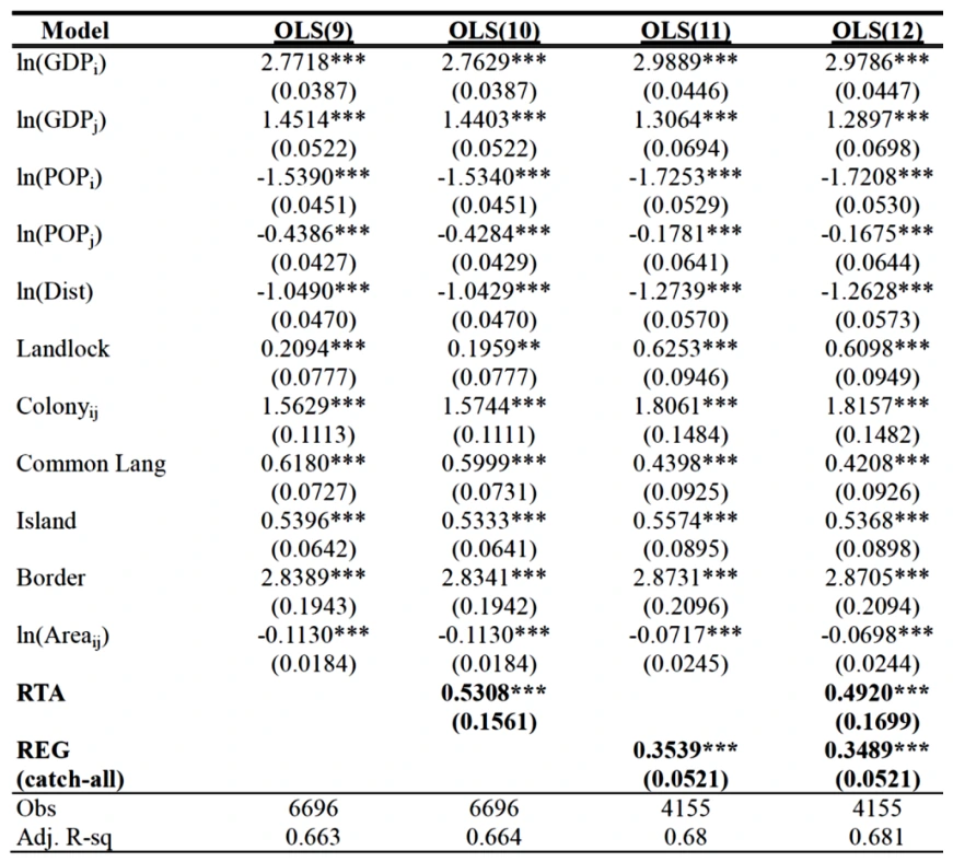
The gravity variables alone fit the model slightly better with adjusted R² = 0.722 for the intra-OECD sub-sample (comparing Models OLS(1) vs. OLS(5)) but only 0.663 for the inter-OECD sub-sample (comparing Models OLS(1) vs. OLS(9)).

We concentrate our discussion on the full baseline models (i.e. Models OLS(8) and OLS(12)). Concerning geographical variables, landlocked economies in the intra-OECD sample do not have any significant results, but it carries a significantly positive impact in the inter-OECD sample. It suggests that a landlocked non-OECD economy attracts more FDI than a non-landlocked one. Island economies on the other hand carry a significantly negative impact on FDI in the intra-OECD sample but a significantly positive impact in the inter-OECD sample. Theoretically, an island economy may reflect a certain level of isolation in the region and thus it may incur higher transport costs for others to access the entity. Nevertheless, having a coastal line of its very own nature may also imply easier access to foreign goods and capital. The effect of being an island economy on FDI is therefore ambiguous, as shown in our dataset. Having a common border significantly determines FDI in the inter-OECD region, whereas such an effect is not significant in the intra-OECD region. In both sub-samples, physical areas are negatively related to FDI. It possibly reflects the higher transport costs from one economic centre to another.

Cultural ties significantly explain bilateral FDI in both samples. If the FDI destination economy and the source were ever in a colonial relationship, the volume of FDI is also likely to be greater. Such effect is comparatively more prominent in the inter-OECD region as expected since there are very few OECD countries ever in a colonial relationship with each other. In contrast, the effects of a common language and having a common coloniser play a more significant role in the intra-OECD sub-sample, demonstrating that the effect of cultural ties is equally played between the rich country pair. All these effects are statistically significant at a 1% level in both sub-samples.

On the variables of our interest – RTA and REG, the baseline specifications using the three sets of samples (i.e. Models OLS(4) vs. OLS(8) vs. OLS(12)) are largely consistent. The coefficients remain statistically significant. Comparing the two sub-samples, we find that the coefficients of REG impose a much greater impact on FDI in the intra-OECD sample than that in the inter-OECD sample. It signifies that the domestic regulatory environment comparatively explains intra-OECD FDI more. Amongst the intra-OECD countries, those with a better domestic regulatory environment are also more likely to attract FDI. In contrast, the coefficient of RTA is slightly bigger in the inter-OECD sample. In other words, for the inter-OECD region, FDI from OECD economies is more responsive to RTA than the domestic regulatory environment of the destination economy.

5.2. Linear Panel Data Regressions

As shown above, all OLS results point to the positive association between regional integration and a favourable regulatory environment with FDI. Nevertheless, as discussed before, pooled regressions ignore country-pair-specific heterogeneity. In addition, this does not take into account multilateral resistance. All these may inflate the coefficients on RTA and REG and lead to a biased inference. Hence, we proceed to undertake our panel data analyses. We start from the most restricted FE and RE models. Comparing the test results between OLS and FE estimates, as well as between OLS and RE estimates allows us to test if the country-pair specific heterogeneity is present or not. Breusch and Pagan Lagrangian multiplier test is used to test the RE estimate against that of OLS. The F-test is used to test the FE estimates against the one from OLS. These diagnostic test results are shown in Appendix Section A.4. Both tests suggest that country-specific heterogeneity cannot be ignored and pooled regressions are therefore not preferred.

Since most of the gravity variables for capturing geographical factors and cultural ties are time-invariant, the FE model cannot assess their effects individually since these characteristics will be absorbed into the fixed effects. Nevertheless, we have still performed the fixed effect estimations for the sake of comparison.

RE and FE estimations with country-pair specific effects and time-specific effects are shown in Table 7 and Table 8 respectively. To compare the results on the gravity variables, we can only refer to the OLS results and RE results obtained. Generally speaking, the magnitudes of the gravity variables in the RE models do not show significant differences as compared to that in the pooled OLS regressions (Models OLS(4) vs. RE(1)). The signs and the magnitudes of the coefficients are largely similar.

However, the coefficients of both RTA and REG systematically become smaller in the RE models, but they remain statistically significant at the 1% level. The coefficients on RTA fell from 0.37 in Model OLS(4) to 0.25 in Model RE(1). The coefficients on REG in the corresponding models decrease even more notably from 0.56 to 0.29.

Typeset table reconstructed from version-of-record PDF page 28. Select the image to open the full-resolution facsimile.

Typeset table reconstructed from version-of-record PDF page 29. Select the image to open the full-resolution facsimile.

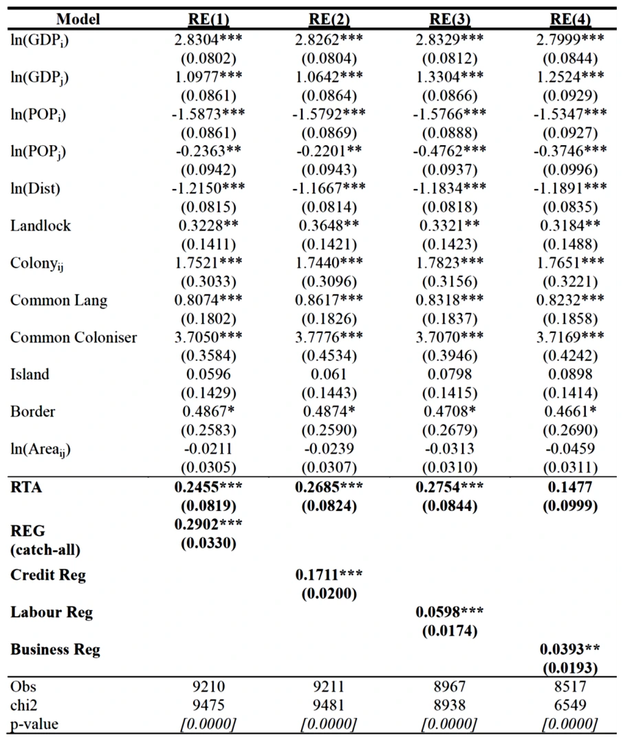
In the panel analysis, we also investigate the impact of three sub-indices of REG, including Credit Reg, Labour Reg and Business Reg on FDI. As shown in Models RE(2) – RE(4), all three measures of regulation stay statistically significant. As expected, the impact of the individual sub-index is less than that of the “catch-all” aggregate measure. Yet the significant results imply that less credit regulations, labour regulations and business regulations in the destination economy are significant determinants of FDI even after controlling for country-pair heterogeneity and other factors of natural barriers. Nevertheless, the coefficients of Labour Reg and Business Reg are much smaller. This may be affected by the reduced sample size due to quite a large number of missing observations for these two sub-indices.

On RTA, the only insignificant coefficient is in Model RE(4). Coefficients in the other three models are quite consistent and comparable. In overall terms, REG explains FDI more than RTA (see Model RE(1)). This implies that generally speaking, the domestic regulatory environment plays a more significant role in attracting FDI than having a regional trade agreement alone.

As discussed earlier, RE models restrictively assume that all the regressors are independent of the unobserved country-pair specific effect. Or else, the results will not be consistent. The results of our FE models suggest that it may be the case for our sample. As shown in Models FE(1) to FE(4), the coefficients of RTA and REG are generally smaller. The coefficients of RTA are even not statistically significant in Models FE(1) and FE(4). For the various measures of the regulatory environment, the broad aggregate REG index remains positively associated with bilateral FDI and so as Credit Reg. However, Labour Reg and Business Reg are no longer significant in Models FE(3) and FE(4).

To verify whether the RE estimations are sensitive to sample selection, RE estimates using intra-OECD and inter-OECD sub-samples are also carried out. Results on the key variables are presented below in Table 9 and Table 10. Compared to Models RE(1) –RE(4), we argue that the key results are not particularly sensitive to the sample selection. REG and Credit Reg of the destination economy are positively associated with FDI. Labour reg is only significant in the intra-OECD sample (i.e. Model RE(7)), but not in the inter-OECD sample (i.e Model RE(11)). It may suggest that labour costs of the developing economies are so low that labour regulation, albeit burdensome, will not hamper FDI. In developed countries, where they do not have comparative advantages on labour costs, labour regulations (i.e. institutional costs) in turn will determine foreign investors’ decisions significantly. Business Reg does not have any significant impact in both sub-samples.

Typeset table reconstructed from version-of-record PDF page 31. Select the image to open the full-resolution facsimile.

Verified table facsimile from source PDF page 31; crop normalised for responsive display.

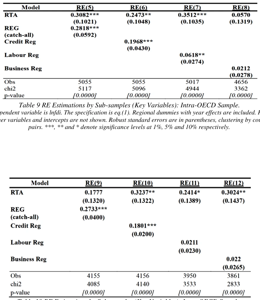
In panel data analysis, the presence of autocorrelation is fairly likely. In this case, the standard errors obtained from the estimates tend to be underestimated, thereby inflating the coefficients. Supported by the test results of Wooldridge (2002)’s autocorrelation test for panel data in Appendix Section A.4, we confirm that the null hypothesis of no autocorrelation can be rejected. In other words, it suggests that the error terms may undergo an AR(1) process. Against this background, FGLS estimation is also carried out. In theory, FGLS estimators are more efficient than RE estimates (which are GLS estimators). We present the coefficients of the key variables in Table 11 below.

Typeset table reconstructed from version-of-record PDF page 32. Select the image to open the full-resolution facsimile.

If we compare the results of Table 12 and Table 13 against Table 14, we note that the coefficients on RTA do not differ a lot even after controlling for heteroskedasticity and AR(1) in the FGLS estimations. For the inter-OECD sample, the effect of RTA lies somewhere between 0.22 to 0.34. For the intra-OECD sample, the corresponding parameter ranges from 0.17 to 0.28. Seemingly, RTA plays a slightly more significant role in attracting FDI in the inter-OECD region than that in the intra-OECD region, after controlling for most of the geographical and cultural factors. However, the difference is very small. In any case, countries having the same membership in a regional trade agreement tend to increase their bilateral FDI.

In terms of the domestic regulatory environment, not only the broad aggregate measure of regulation has a positive and statistically significant impact on bilateral FDI, but so do its sub-indices. Perhaps except for business regulation, its coefficient is relatively small as compared to that of credit market regulation and labour regulation. The inter-OECD sub-sample even shows no significant effect. We reckon that it is very likely due to data limitations. Unlike the other two sub-indices which have reasonably good coverage in the sample period, more comprehensive coverage of business regulation is only available since 2000. The sample size is inevitably greatly reduced.

Comparing the effects of the domestic regulatory environment in the intra-OECD region vis-à-vis the inter-OECD region in Table 11, we find consistently that the effects of regulation are stronger in the intra-OECD region. It may suggest that, in the inter-OECD region, the non-OECD economies have comparative advantages in production costs. Despite their institutional inadequacy, they still have locational advantages in attracting foreign capital. However, amongst OECD economies, comparative advantages do not lie in production costs. Institutional differences would turn out to be a more significant factor to be considered by foreign investors.

Furthermore, we can also note that credit market regulations exert the largest effects on FDI among the three types of regulations. These results are also consistent with the IMF (2005)’s view that one of the most prominent constraints for foreign investors is credit constraints.

A final extension of our linear panel data model before we proceed to IV estimation is to test our specification using Hausman and Taylor estimator. We are aware that there is no prior reason to justify that the correlation between the regressors and the unobserved country-pair heterogeneity does not exist. In addition, our FE models are supported by the test results of Hausman specification tests (see Appendix Section A.4) instead of RE models, suggesting that we cannot reject that the country-pair specific effects correlate with the regressors. As a robustness check, henceforth, we further relax this assumption and employ the Hausman and Taylor estimators in order to accommodate time-invariant variables as well as to allow the unobserved country-pair specific effects to be correlated with the regressors. In our case, we assume that REG and RTA are correlated with the unobserved country-pair-specific effects.

Table 12 to Table 14 shows our Hausman and Taylor estimation results using the full sample, inter-OECD and intra-OECD sub-samples respectively. After using Hausman and Taylor estimators, different geographical variables behave differently in the two subsamples. Basic gravity variables, e.g. GDP, population and distance between the two economies, have the expected signs. Other than that, being an island economy is negatively affecting FDI inflows in the intra-OECD region. However, such an effect is not found in the inter-OECD region. Having a common border positively explains FDI between two economies, but this effect is not statistically significant in the intra-OECD sub-sample. Area product is not significant at all in both sub-samples. In overall terms, geographical variables do account partially for bilateral FDI. However, the effects of specific geographical characteristics will differ slightly in the inter-OECD and intra-OECD regions.

In terms of cultural linkages, similar to the qualitative results obtained from our OLS estimates, we find that the effect of common language is significant in determining bilateral FDI. The effect, however, primarily comes from the intra-OECD sample. In other words, for OECD economies, whether the destination economy has a common language as the source is not a statistically significant determinant when they consider the outward investment in non-OECD economies. However, if the destination economy is also an OECD economy, such a factor will be significant. For the inter-OECD region, such sort of cultural proximity may have been captured by the colonial relationship variable instead of the common language variable. We find that in the inter-OECD region if the FDI source and destination economies are ever in a colonial relationship, they are more likely to have more bilateral FDI.

The positive and significant impacts of RTA and REG survive even if we use Hausman and Taylor estimators. The results still hold after using sub-samples. Concerning the individual regulatory sub-index, only credit market regulations are statistically significant throughout. Labour market regulations and business regulations are not significant in either sub-sample. This reiterates earlier results that an economy with less regulated credit markets fosters a more favourable business environment, thereby inducing more inward investment.

Typeset table reconstructed from version-of-record PDF page 35. Select the image to open the full-resolution facsimile.

Typeset table reconstructed from version-of-record PDF page 36. Select the image to open the full-resolution facsimile.

Typeset table reconstructed from version-of-record PDF page 37. Select the image to open the full-resolution facsimile.

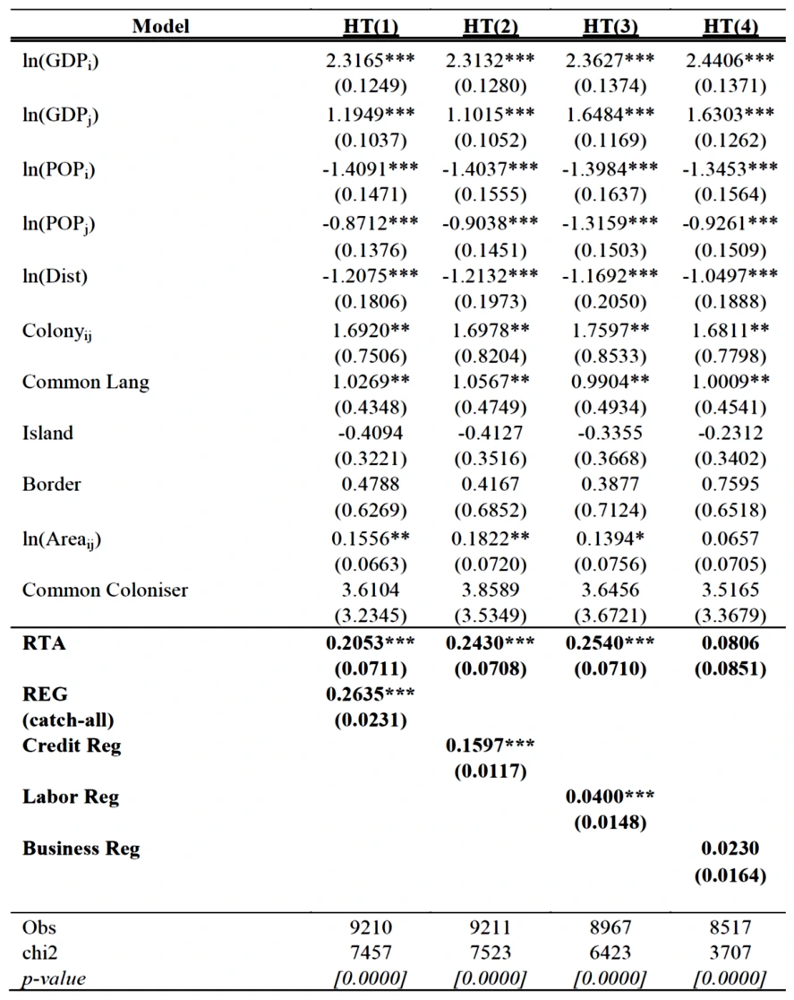
To sum up, so far, we use several linear panel data estimators to assess the effects of natural barriers, RTA and regulatory environment on bilateral FDI in an augmented gravity model. The various estimators have their own merits and shortcomings. Despite so, the qualitative conclusion is largely similar. Our empirical findings suggest that the gravity model fits our data fairly well. Geographical characteristics and cultural ties are essential FDI determinants, although they are not particularly robust to different samples used. More importantly, both external institutions – RTA and the domestic regulatory environment are also significant determinants of bilateral FDI in both the intra-OECD and inter-OECD regions.

This conclusion is encouraging from the economic development perspective. While we understand that FDI is growth-promoting, we provide empirical evidence to support that improving the regulatory environment and being actively engaged in regional integration are two possible channels to promote FDI. More specifically, relaxing credit market regulations carries even more pronounced impacts. These results have been controlled for physical and historical elements, like geography and culture, which are time-invarying and deterministic.

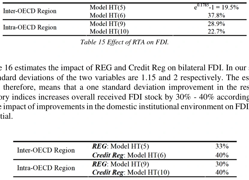
To quantify the results we have for easy reference, the following tables show the impact of our key variables on FDI based on the Hausman and Taylor estimators. Table 15 shows that if a source country k has a mutual membership of RTA with a destination country j, it is estimated that j would receive around 19.5% to 37.8% more FDI stock from country k. The magnitude depends on whether country j is an OECD economy in our case.

Typeset table reconstructed from version-of-record PDF page 38. Select the image to open the full-resolution facsimile.

Verified table facsimile from source PDF page 38; crop normalised for responsive display.

Finally, along the line of the existing literature on institutions and growth, we tackle the potential endogeneity problem between regulation and FDI by means of IV estimation. More specifically, we use Baltagi (1981)’s, EC2SLS estimator. The hypothesis is that destination economies with a less burdensome regulatory environment will be more likely to attract FDI. Simultaneously, more FDI may also induce structural reform to improve the business environment by reducing regulations.

Before we discuss the IV estimation results, we deploy the Hausman specification test to test whether various measures of regulation correlate with the disturbance terms in our models. Test details are in Appendix Section A.4. The test results suggest that there is no evidence to show REG and Labor Reg are endogenous variables. However, Credit Reg and Business Reg do correlate with the disturbance terms. With the absence of endogeneity, using IV estimates or least square estimations yield consistent results. However, if endogeneity does exist, only IV estimators provide consistent results. In any case, we perform IV estimators for all 4 indices of the regulatory environment to facilitate comparison.

Following Alesina, et al. (2003) and Bénassy-Quéré, et al. (2007), we consider using ethnic fragmentation, religion fragmentation, the latitude of the economy and the UK legal origin of the destination economies as instruments. Sargan-Hansen test, as shown in Appendix Section A.4 and the results tables follow, supports that our instruments used are relevant.

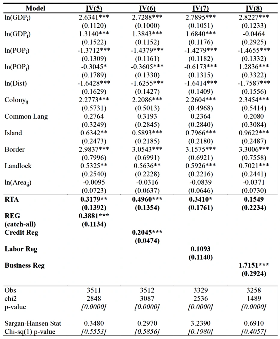
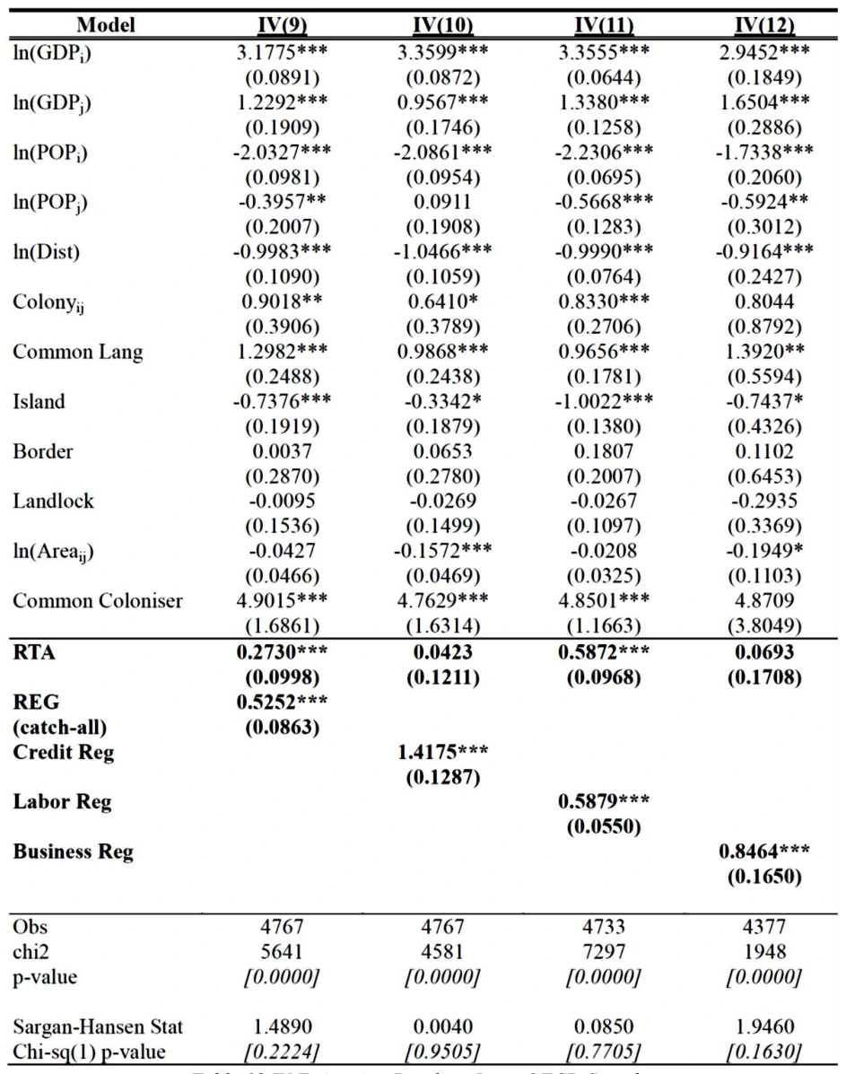
The estimation results using panel EC2SLS for the full sample and sub-samples are shown in Table 17 – Table 19. Key gravity variables (GDP, population and distance) and variables measuring cultural and historical ties remain significantly associated with bilateral FDI. Other geographical variables such as area, common border and island economy are no longer significant. However, their effects are statistically significant in different sub-samples and behave differently.

On the effects of RTA, the results using the full sample show that the coefficients of the IV estimations are systematically larger than those previously obtained in various linear models, for example in the RE models (i.e. Models IV(1) – IV(4) vs. RE(1) –RE(4)). Comparing the coefficients of RTA of the intra-OECD sample (i.e. Models IV(9) – IV(12)) vis-à-vis the inter-OECD sample (i.e. Models IV(5) – IV(8)), the results generally suggest that RTA exerts stronger impact on inter-OECD bilateral FDI.

The overall impact of regulation also turns out to be more significant in Models IV(1) – IV(4) after controlling for endogeneity. One point to note is that the “catch-all’ index of REG consistently has larger coefficients than those of RTA in the full samples and both sub-samples.

With respect to the three sub-indices, we find that the effects of both Credit Reg and Business Reg are statistically significant in both sub-samples (i.e. Model IV(6) vs. IV(10) and Model IV(8) vs. IV(12) respectively). The effect of credit market regulation is more profound in the intra-OECD sample, whereas the effect of business regulations is greater in the inter-OECD sample. Labour Reg, on the other hand, only associates positively with FDI in the intra-OECD sample (i.e. Model IV(11)), whereas such an effect is not statistically significant in the inter-OECD sample at all (i.e. Model IV(7)). In sum, we find empirical evidence to show that the regulatory environment positively and significantly relates to bilateral FDI, in particular in the intra-OECD region.

One may wonder if RTA is also a potential endogenous variable, such that economies with more bilateral FDI flows in between are more likely to engage in an RTA or vice versa. However, as Rose (2004) reckons, there is no theoretical basis for choosing an appropriate instrument for RTA. Despite so, we have attempted to use the same instruments as in our IV estimations for considering both RTA and regulation as endogenous. Nevertheless, the Sargan-Hansen test rejects the validity of the instruments for RTA. Hence, we do not show this set of IV estimations here.

In sum, we find that even having considered the potential endogeneity problem of regulation, our qualitative conclusion does not change. That said, regional integration and the regulatory environment of the destination economy do matter for bilateral FDI. However, we should note that our IV estimation results tend to inflate the coefficients of the variables of our key interest when compared to those obtained in our linear panel data models. Although the Sargan-Hansen test supports the validity of our instruments, we should be very cautious when interpreting the IV estimation results.

Typeset table reconstructed from version-of-record PDF page 41. Select the image to open the full-resolution facsimile.

Typeset table reconstructed from version-of-record PDF page 42. Select the image to open the full-resolution facsimile.

Typeset table reconstructed from version-of-record PDF page 43. Select the image to open the full-resolution facsimile.

6. Conclusion

In this paper, we investigate the impacts of natural barriers, “at-the-border” regional integration and the domestic regulatory environment in the destination economy on FDI. Our study demonstrates that all three factors do matter for bilateral inward FDI stock.

The existing literature argues that the favourable institutional quality of the destination economy attracts more FDI. Nevertheless, these studies are usually based on crosssectional data. Not only is the use of panel data limited, but country-specific characteristics of the source and destination economies also are not controlled simultaneously. Furthermore, there is not yet any study specifically devoted to the impact of the domestic regulatory environment on FDI. On the impact of regional integration on FDI, as proxied by mutual membership in an RTA, earlier studies show mixed results. We are also interested in examining the impact of such external institutions vis-à-vis domestic institutions on FDI.

We use a bilateral FDI stock dataset of 60 FDI destination economies sourcing from OECD economies during 1985 - 2006. The augmented gravity framework fits our data quite well. Our empirical results suggest that geographical, historical and cultural factors generally explain bilateral FDI significantly, even after controlling for unobserved country-pair heterogeneity and time effect. However, the effects of geographical determinants on FDI are differently felt in the intra-OECD and inter-OECD regions.

Panel data analysis shows that a lax regulatory environment and an RTA are positively associated with inter-and intra-OECD bilateral FDI. These qualitative results survive when we use different estimation techniques, including FE, RE, FGLS and Hausman and Taylor estimations. All sub-indices of regulation show the results that a less burdensome regulatory environment is favourable to FDI. With regard to a specific type of regulation, the results of credit market regulations are most robust to different estimators. Results on labour market regulation and business regulation, though positive, are insignificant in some cases. These results on one hand suggest that credit market constraints are perhaps one of the key concerns for foreign investors. This also echoes the view that financial development is important to economic development (amongst others, see Rajan and Zingales (1998)). On the other hand, labour market rigidity and business regulation may not be such prime concerns for foreign investors as one anticipates. According to our Hausman and Taylor estimation results, engaging in an RTA could lead to more bilateral FDI stock by 19.5%-37.8%. Improving the domestic regulatory environment by, say, around 1.5 to 2 points in our sample, bilateral FDI stock could increase by some 30% to 40%.

To investigate the potential endogeneity problem of regulation, we also carry out IV estimation. For the inter-OECD region, RTA is significantly associated with FDI and shows a more significant impact than that in the intra-OECD sample. For the intra-OECD region, the regulatory environment of the destination economies plays a more significant role. Indeed, using IV estimations reinforces further the significance of the regulatory environment of the destination economy in attracting FDI than the results obtained in panel data linear models where endogeneity is not accounted for.

Regionalism remains a key issue, in particular during the financial turmoil the world is experiencing. Despite global trade imbalances, world leaders remain committed to preventing the surge of protectionism. The empirical results presented here may add some support to this commitment. Regionalism does not only foster trade. As shown here, it also leads to more FDI. Furthermore, it also strengthens the investment linkage between groups of economies with different stages of economic development and institutional environments.

As a strategy for long-term growth, domestic structural reform efforts have been made across the board to improve domestic institutional frameworks so that the efficient functioning of markets can be supported. Our sub-sample analysis also demonstrates that even amongst the developed economies (i.e. the intra-OECD sample), the regulatory environment still plays a significant role in-attracting foreign capital. In particular, when the comparative advantages of the economy do not lie in the production costs, institutional strengths and differences turn out to be more essential in affecting foreign investors’ decisions. As shown in our findings, the regulatory environment affects intra-OECD bilateral FDI equally as (or even more than that) in the inter-OECD sub-sample.

From a policy implication perspective, this paper highlights the importance of removing “behind-the-border” regulatory barriers to attract foreign investment irrespective of the stage of development of the economies. In our work, we nevertheless do not provide enough evidence to conclude that RTAs are necessarily desirable. In particular, we have not considered the cost and trade diversion brought about by RTAs. However, our findings support that promoting regional integration may also open up a channel of development, i.e. to attract FDI.

Limitations

In our work, we nevertheless do not provide enough evidence to conclude that RTAs are necessarily desirable. In particular, we have not considered the cost and trade diversion brought about by RTAs. However, our findings support that promoting regional integration may also open up a channel of development, i.e. to attract FDI.

About the Research

This series is composed of five papers (The new version of the papers was created from my MPhil thesis), one is an overview and four empirical studies, which investigate the effects of institutions on cross-country economic development from different perspectives drawn from my MPhil thesis of "Essay on Institutions, Policies, and Economic Development". The first paper, entitled "Institutions, Policies, and Economic Growth Overview", reviews the relationship between institutions and policy regulation with economic development from the perspective of economic literature. The second paper, entitled “Impact of Institutions and Policy on Economic Growth: Empirical Evidence", empirical analysis to explore the interaction between the institution and economic development. The third paper, entitled “Role of Political Institutions on Economic Growth: Empirical Evidence”, is an empirical analysis to explore the effect of political institutions on economic development. The fourth paper, entitled “Impact of Natural Environment, Regional Integration, and Policies on FDI”, explores the effects of three determinants of bilateral FDI, including natural barriers, the “at-the-border” barrier (regional trade agreement), and the “behindthe-border” barrier (domestic regulatory environment). The fifth paper, entitled “Cross Countries Economic Performances - SPF Approach”, explores the differences in technical inefficiency (inefficient allocation of production inputs) and explains the diverse cross-country economic performances, using estimating a “global” stochastic production frontier (SPF) mod.

APPENDICES

A.1 Component of the Regulation Index (REG). Descriptive Statistics and Correlation

Matrices

Components of the Regulation Index (REG) of the Fraser Institute’s Economic

Freedom of the World Report

A. Credit market regulations (Credit Reg) i. Ownership of banks: percentage of deposits held in privately owned banks ii. Competition: domestic banks face competition from foreign banks ii. Extension of credit: percentage of credit extended to the private sector iii. Avoidance of interest rate controls and regulations that lead to negative real interest rates

B. Labor market regulations (Labour Reg) i. Impact of the minimum wage: the minimum wage, set by law, has little impact on wages because it is too low or not obeyed ii. Hiring and firing practices: hiring and firing practices of companies are determined by private contract iii. Share of labour force whose wages are set by centralized collective bargaining iv. Mandated cost of hiring iv. Mandated cost of worker dismissal v. Use of conscripts to obtain military personnel

C. Business regulations (Business Reg) i. Price controls: extent to which businesses are free to set their own prices ii. Administrative conditions and new businesses: administrative procedures A are an important obstacle to starting a new business iii. Time with government bureaucracy: senior management spends a substantial amount of time dealing with government bureaucracy iv. Starting a new business: starting a new business is generally easy v. Extra payments/bribes: irregular, additional payments connected with import and export permits, business licenses, exchange controls, tax assessments, police protection or loan applications are very rare vi. Licensing restrictions: Time in days and monetary costs required to obtain a license to construct a standard warehouse vii. Cost of tax compliance: Time required per year for a business to prepare, file, and pay taxes on corporate income, value-added or sales taxes, and taxes on labour.

Source: Gwartney, et al. (2008)

Descriptive Statistics of Institutional Variables

Correlation Matrix of Institutional Variables

A.2 List of Economies

Country Coverage

A.3 List of Regional Trade Agreements (RTA)

A.4 Diagnostic Tests for Estimations F-test for FE vs. OLS Estimations

I. F-test for FE vs. OLS Estimations

An F-test is used to test for the existence of individual effects. The test for the two-way error component model is similar to the one-way model. Given time effects, the null hypothesis assumes

The unrestricted residual sum of squares (URSS) is within the residual sum of squares.

However, the restricted residual sum of squares (RRSS) is based on the regression

The F-ratio used for the test is

where k is the number of regressors. F-test results of our FE models are presented below:

Note: Conclusion does not change when using inter-OECD and intra-OECD samples.

II. Breusch and Pagan test for RE vs. OLS Estimations

Breusch and Pagan's test results on the RE models are shown below:

III. Hausman Specification Test

The specification test devised by Hausman (1978) is used to test for the orthogonality of the common effects and the regressors. The test is based on the hypothesis of no correlation. Under the null hypothesis, both OLS estimations in the FE model and GLS in the RE model are consistent, but OLS is inefficient. Under the alternative, OLS is consistent, but GLS is not. Therefore, under the null hypothesis, the two estimates should not differ systematically. The covariance matrix of the difference vector (𝑏−𝛽^̂)

Where 𝑏 𝑎𝑛𝑑 𝛽^̂ are estimates obtained from OLS and RE respectively. Hausman’s result is that the covariance of an efficient estimator with its difference from an inefficient estimator is zero, which implies

The chi-squared test is based on Wald’s criterion:

For 𝛹^̂, one can use the estimated covariance matrices of the slope estimator in the FE model and the estimated covariance matrix in the RE model, excluding the constant term. Under the null hypothesis, W has a limiting chi-sq. distribution with K – 1 degree of freedom. Hausman specification test results on the four key baseline panel models are as shown below:

Note: Conclusion does not change when using inter-OECD and intra-OECD samples.

For IV estimation, the Hausman specification test can also be used to test whether REG is endogenous, i.e. correlated with the disturbance term in our model. Under the null hypothesis, there is no correlation between the two. If this is the case, estimators of both least squares and IV are consistent. Under the alternative hypothesis, only the IV estimator is consistent.

IV. Test for Autocorrelation

Wooldridge’s procedure begins by estimating the parameters β¹ by regressing ∆y^it on ∆X^it and obtaining the residuals êit. If the εit are not serially correlated, then Corr(∆ε^it, ∆ε^it−1) = −0.5. Given this, the procedure regresses the residuals êit from the regression with first-differenced variables on their lags and tests that the coefficient on the lagged residuals is equal to −0.5 by using F-test. Our test results are below. The null hypothesis of no serial correlation is strongly rejected.

Note: Standard errors account for clustering within the panels. The conclusion does not change

when using inter-OECD and intra-OECD samples.

V. Sargan-Hansen Test on Instruments Validity

A Sargan-Hansen test of over-identification restrictions is used to test the homogeneity of the instruments, i.e. the instruments are uncorrelated with the error term, and the excluded instruments are correctly excluded from the estimated equation. In short, under the null hypothesis, the instruments are valid. The test results are shown in the IV estimation results table in Table 17 – Table 19. The test results conclude that we cannot reject the homogeneity of the instruments.