 Journal of Global Trade, Ethics and Law
1. Introduction
Concerns about the de-globalization after the global financial crisis (GFC) of 2008 (Garcia-Herrero, 2019; and Evenett and Fritz, 2021), heightened by the US-China trade war and increasing use of non-tariff measures (NTM) and subsidies in recent years, are growing. A joint paper by the staff of International Monetary fund (IMF), Organization for Economic Cooperation and Development (OECD), World Bank (WB) and World Trade Organization (WTO) notes: “Subsidies appear to be widespread, growing, and often poorly targeted at their intended policy objectives. Beyond raising economic efficiency concerns, this situation is spurring the use of unilateral trade defense measures, eroding public support for open trade, and contributing to severe trade tensions that impede progress on other global trade priorities. Governments should work expeditiously to clarify and strengthen international disciplines around subsidies while recognizing the important roles that well-designed subsidies can play in some circumstances” (IMF, OECD, WB, and WTO, 2022). Whether the national Governments will oblige, given the crisis in the global governance system (Lavdari, 2022), is open to question. In this backdrop, the evidence that the actions of the countries concerned are inimical to their own interests might lead to an effective solution of the problem. This paper is guided by this thought.
“Protectionism arises in ingenious ways. As free trade advocates squelch it in one place, it pops up in another” (Bhagwati, 2008). In the context of the 2018 tariff actions by the US and the retaliation by its major trading partners, and the perceived inability of the ‘profession’, despite two centuries of intellectual work, to persuade the ‘public’ about the merits of free trade, it is conjectured that “perhaps some of the public’s mild views on protectionism stem from the fact that most of economic analysis of protectionism is theoretical, microeconomic or dated” (Furceri et al, 2019). Empirical, macroeconomic or updated analysis may not be the solution; the analyst would need to walk the extra mile and explain how protectionism impacts home country economic activity amid other factors at play.
India is a special case. The country needs and is striving for rapid economic growth. Apart from the macroeconomic stability that provides an enabling environment, the thrust on capital expenditure (CAPEX) for creating physical infrastructure (Sood et al, 2022 and 2023) and the efforts made by the Government of India (GoI) to improve the performance of domestic manufacturing merit a mention. The Government also implemented several growth-supportive regulatory reforms (Panagariya, 2018 and 2020). These apart, policy measures from the toolkit of the Reserve Bank of India (RBI) and GoI were used to fight the assumed short-term economic slowdown (GoI, 2020; RBI, 2020). Protectionism, along with a few policy-related systemic problems, is thwarting the efforts. This is the central message of this paper. Protectionism thrives in India either due to the theoretical beliefs about its benefits or due to the fact that the policy debate is often rife with presumptions that drive the policy attention away from the larger issues. The theoretical aspects are discussed later. This Section revisits the recent policy debate and puts the spotlight on the elephant in the room.
India ranked 90th in the 2021 International Trade Barriers Index brought out by THOLOS Foundation that identifies the most direct and indirect trade barriers imposed by 90 countries (affecting 95% of world GDP) indicating that India imposes most of the trade barriers (Thompson, 2021). The simple average ‘most favoured nation’ tariff (SAMT) on all products of 18.3% in 2021 in India was among the highest in the world. India is the fourth largest user of NTM in the world, after China, US and Thailand. The absolute size of budgetary support to agriculture in India is the fourth largest, after the ‘European Union (EU) with UK’, US and China. In relative terms, the budgetary support to agriculture (18% of gross farm receipts) places India in the company of a handful of advanced economies (IMF, OECD, WB, and WTO, 2022). India is now into corporate subsidy with the production linked incentive (PLI) scheme from 2020. These facts grab the headlines. What is less discussed is that tariffs increased in India from 2011 (sharply from 2018), a de-facto reversal of the tariff reforms done during 1992-2008. This and the large number of anti-dumping procedures initiated (ADPINI) by India make it a phenomenon of foreign trade on the reverse gear (FTRG), the subject matter of this paper.
1.1. India’s Growth Imperatives and Policy Debate
India – home to 18% of the global population with 3% global income in current US$ in 2021 [7% in purchasing power parity (PPP) current international $]1 – ranked 132 (out of 191 countries) in the human development index in 2021/2022 [United Nations Development Programmes (UNDP, 2022)]. Developmental efforts need to be intensified, and the urgency of rapid economic growth in this country cannot be overstated. The announcement by Prime Minister Narendra Modi on August 15, 2022, of the goal to make India a developed country by 2047 has ignited a debate on the economic growth imperatives in India. In keeping with World Bank’s classification of countries in terms of income levels, India’s gross domestic product (GDP) per capita needs to grow by about 7% per annum for a “full generation” (from $2,170 in 2021) to reach the level of $13,205, the current threshold for the high-income country group; and India’s annual per capita income (PCI) growth of 4.3% over the past generation was nowhere near to the required rate (Eberstadt, 2022). Korea with a PCI of PPP $17,810 (2011 prices) was admitted as an OECD member in 1996; India’s PCI (PPP $6,067 in 2021-22) can reach the level of a developed country (PPP $18,000) if it grows at 4.1% for the next 26 years (Bhalla, 2023). As “2047 is not 1996”, India needs a higher benchmark (Kumar, 2023). Kumar provides two alternatives: (a) PCI grows from the current level of $6,592 (at constant 2017 international $) to $44,827 by 2047 for India to be a full-fledged OECD member; it requires a PCI growth of 7.95% for 25 years or GDP growth of about 8.6% (taking a population growth of 0.7%). (b) Since this growth may seem “unrealistic”, India can target a PCI level of $33,106 (average of half of the current OECD members); for this, India’s PCI needs to grow at 6.7% (GDP at 7.4%).
1 Sourced from World Development Indicators (WDI) database of WB. Current US$ is relevant for international transactions. PPP is also used in international comparison of income levels.
Some 10-15 years ago, with the trend growth of India at 8% just before the GFC (Anand et al, 2014), policymakers would take 8-9% growth for granted. Why the 8.6% growth would seem unrealistic now? Is it because the trend rate has fallen (Sheel, 2022)? If yes, why that happened? These questions are important. This paper makes an attempt to find the answers.
What is the outlook on growth at present? Several structural reforms done during the last eight years have laid India on a stronger foundation for higher rate of growth (Kumar, 2023). A 2023 book has the antithesis. The book makes the crucial point that the Governments have neglected the provision of public goods for shared progress: education, health, functioning cities, a fair judiciary and a clean environment (Mody, 2023). The concerns regarding public goods are shared by many, although the policy perspectives vary (WB, 2004; UNDP, 2019; Ho, 2019; Balakrishnan, 2022). In particular, education in India is in a deplorable state and the position likely has worsened in recent times (discussed later in this Section and in Section 4).
The surmise that the recent reforms would take India on the high growth path is not fully assisted by the data. Conceptually though, regulatory reforms, by making the doing business easier, promote growth (De Soto, 2000; WB, 2020), and policy uncertainty retards growth (Baker et al, 2016; Bhagat et al, 2016; Wei, et al, 2021). In India, the subdued pace of economic growth during 2012-14 is popularly attributed to the “policy paralysis” in the then government. Empirical studies attribute it to “heightened regulatory and policy uncertainties, delayed project approvals and implementation, continued bottlenecks in the energy sector as well as reform setbacks, contributing to a lower investment rate and sluggish TFP growth” (Anand et al, 2014), or a “regression to the mean” in the growth (Pritchett and Summers, 2014) or “cyclical downturn” (Patnaik and Pundit, 2014). With a new government in place from 2014, several reforms were implemented, and India’s position in WB’s doing business ranking improved from 134th in 2014 to 63rd in 2020. GDP growth improved from 6.4% in 2013-14 to 8.3% in 2016-17, but fell to 3.9% in 2019-20 despite the reforms and no ‘policy uncertainty’.2
Several explanations are available about the growth slowdown of 2017-20, the foremost among them being the demonetization (withdrawal of two large value currency notes from circulation) on November 8, 2016, and implementation of Goods and Services Tax (GST) on July 1, 2017 (Nagaraj, 2020; Balakrishnan, 2022; Mody, 2023). The slowdown (initially observed during 2016-18) was a “display of weak spots in macro data”: studies using alternative data (such as ‘nightlight’) show that demonetization adversely impacted economic activity; this evidence is fine, but the problem comes when it is used to gauge the macro-level impact (Mallik, 2018). In revised data, GDP growth improved to 8.3% in 2016-17 from 8% in 2015-16. Growth decelerated from 2017-18. It is difficult to say how much of it was due to the demonetization or GST, given the wide variety of explanations available – the slowdown was cyclical, structural, both cyclical and structural, due to the ‘four balance sheet problem’, ‘drag of the financial sector on the real sector’, ‘weak demand’ or a ‘contractionary macroeconomic stance’ of the GoI (Lahiri 2019; Subramanian and Felmen 2019; GoI, 2020; Mukhopadhyay, 2021;
2 India’s fiscal year is on April-March basis. The growth rates cited in the paper are year-on-year at constant national prices, unless specified otherwise.
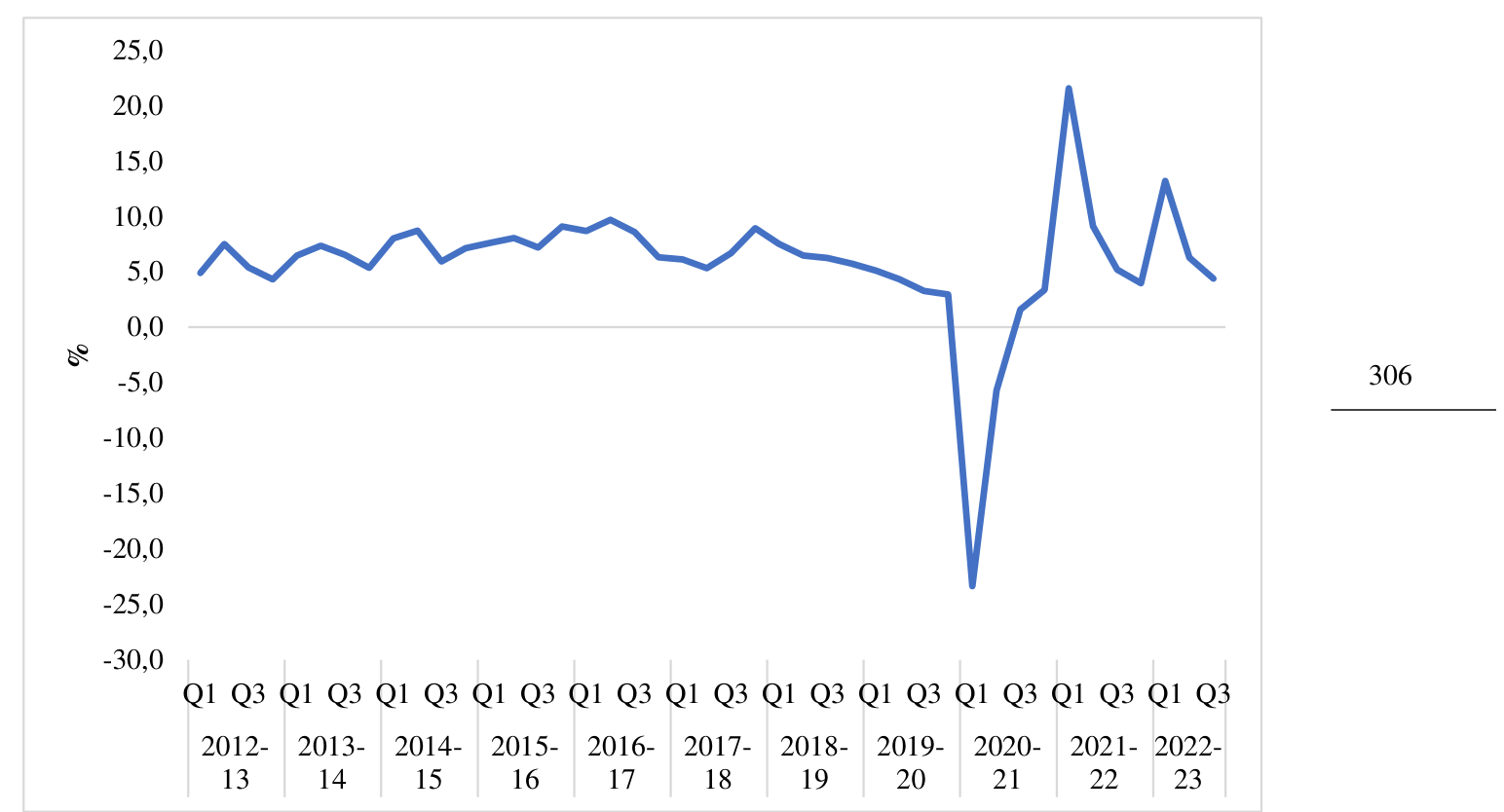
Balakrishnan, 2022). Policy actions (including monetary easing and reduction in corporate tax rates) to address the concerns didn’t help. GDP growth fell for eight quarters in a row from 8.9% in Q4:2017-18 to 2.9% in Q4:2019-20. After oscillating from Q1:2020-21 to Q1:2022-23 due to imposition/relaxation of pandemic related restrictions, growth was trending towards the pre-pandemic low (Fig 1), suggesting that the problem is enduring.
A related issue is the weak show of manufacturing despite the supports extended by the GoI. The ‘Make in India’ initiative launched in 2014 aimed at raising its share in GDP to 25% by 2020 (from about 15% in 2014). The sector’s share fell to 13.5% in 2019, sliding further to 13.3% in 2022; these were close to the low of 1967 (Fig 2) reviving memories of the industrial stagnation from the mid-1960s through the 1970s (Ahluwalia, 1985; Nayyar, 1994).

1.2. The Elephant in the Room
There are three major problems. One, imports are curbed, while most of India’s imports are industrial inputs in some form or the other.3 Two, an economy that industrialises should be able to move from importation to absorption and adaptation of technology though innovation (Nayyar, 1997, 361); research and development (R&D) expenditure (% of GDP) declined in India after 2008, unlike the increase in other countries (discussed in Section 4). Three, investment in human capital is a “pervasive phenomenon” (Becker, 1962, 49); in India, about 25% of the rural youth in the 14-18 age group cannot read basic text fluently in their own language, and more than half struggle with division (3 digit by 1 digit) problem, although 86% of the youth in this age group were within the formal education system (Pratham, 2017]. The position likely has worsened as schools are running with acute shortages of teachers and several other problems [United Nations Educational, Scientific and Cultural Organization (UNESCO), 2021]. The quality of instruction and learning outcomes are low in many countries (WB, 2004); the problems in India are basic: (a) it’s “no teacher, no class” as the caption of UNESCO (2021) report puts it; and (b) public expenditure on education (as a % of GDP) is small (in global comparison), and a relatively large portion of it goes for higher education (Balakrishnan, 2022).
All the three would hurt productivity, exports and GDP growth. Import curbs reduce the availability of inputs for user industries and lessen competition in domestic product market. Decline in R&D expenditure relative to GDP leaves India behind others technologically. India produces 15 lakh engineers per year (Aiyar, 2023); macro level productivity will depend on the work done by the entire work force (543 million in 2022, as estimated by Bhalla and Das, 2023), where basic education matters. And productivity is crucial for the success in exports.
3 Capital goods, intermediate goods and raw material together accounted for 87% of the total value of India’s merchandise imports in 2019 (World Bank, WITS database).
1.3. Research Methodology and Contribution to the Literature
This paper examines these propositions using macro-level data for 1980-2020 period by deploying four autoregressive distributed lag (ARDL) models on imports, productivity, exports, and GDP.4 The imports model captures the impact of import curbs on import demand. The impact of competition in domestic product market attributable to import curbs is captured in productivity- and exports models. The GDP model captures the impact of exports, non-oil imports and education. Diagnostic tests confirm the robustness of the models estimated. Granger causality tests (done to ascertain the direction of causality between select variables, where it’s not a settled proposition) corroborate the findings. Reinforcing the evidence from the ARDL models and invalidating the received wisdom, sectoral data show that the 2017-20 economic slowdown owed it to import curbs. Cross country data and information on two manufacturing industries in India elucidate that the tariff/subsidy support may not enable domestic activity to endure the de-globalization. The stylized patterns on export performance and GDP growth in independent India, covering two spells of FTRG (1956-75; 2012-20) and one when it was foreign trade on the front gear (FTFG) (1987-2012), reinforce the points.
The paper contributes to the policy debate on economic growth in India and addresses the global concerns about the de-globalization. The methodology used in the paper helps in explaining how the import curbs impact economic activity amid other factors at play, and it differs from the conventional measurement of short/medium-term impact of tariff on economic growth or welfare loss (e.g., Furceri et al 2019; Fajgelbaum et al, 2020; Ding et al, 2022).
The rest of the paper is organised into five Sections. Section 2 documents the evidence on the reversal of tariff reforms in India and presents a brief review of literature on the growth impact of tariff. Section 3 describes the research methodology. Section 4 discusses the findings. Section 5 specifically addresses the question as to why the Government support does not improve the performance of Indian manufacturing. Section 6 concludes.
4 Periods covered in individual ARDL models vary depending on the availability of data on crucial variables.
2. Reversal of Tariff Reforms
India pursued an inward-looking policy regime during 1950-75.5 Import-substituting industrialization gave rise to more expensive and lower quality products than what could be imported, and this impacted the exports. Ad-hoc liberalization measures were initiated during 1976-1991. The period from 1992 saw deeper and systematic trade policy reforms (Bhagwati and Desai, 1970; Bhagwati and Srinivasan, 1975; Ahluwalia, 1985; Panagariya, 2004).
SAMT declined in India from 84.1% in 1990 to 12.8% in 2008 moving closer to the global average (9.9%). After the GFC, the global average fell to 8.9% in 2017, but Indian tariff stayed around the 2008 level till 2010 and then rose to 13.8% in 2017. When others, especially the low & medium income (LMY) countries, continued tariff reduction, India didn’t (Table 1).

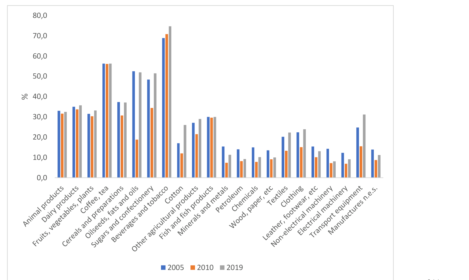
According to the WTO, the SAMT in India rose to 17.6% in 2019. The five percentage points increase in the SAMT in India between 2010 and 2019 was incidentally a global record. Data for 22 major product groups show that the tariffs in 2019 were generally higher than the levels of 2010, some even surpassing the level of 2005 (Fig 3).6 The High-Level Advisory Group (HLAG) set up by the GoI flags the recent increases in India’s tariff: “this trend needs to be arrested and reversed” (GoI 2019, 12). To the contrary, the subsequent budgets raised tariffs on many products. Reversal of trade liberalisation “increasingly appears to be a firmly established policy of the government” (Panagariya, 2022a).
5 This is a broad generalization of the policy regime: there were differences in the perceptions about foreign trade in the planning process (Nayyar, 1997).
6 There are differences in tariffs across datasets. Illustratively, India’s SAMT in 2019 was 15.5% in WDI database of the WB while it was 17.6% in WTO data. WDI data on country-groups (available up to 2017) are given in Table-1. Data used in the econometric models are also from WDI. Product-group wise tariffs are from WTO.
2.1. Literature on Growth Impact of Tariff
In the classical era, tariffs would reshuffle the fully employed workforce. The Keynesian case for protection, in periods of unemployment, is on the premise that tariffs would divert aggregate demand from foreign to domestic goods. Later advances in the literature show that tariffs under flexible exchange rates have a contractionary effect on output, with the implication that countries with flexible exchange rates should rely more on monetary and fiscal policy to correct large-scale unemployment (Mundel, 1961; Krugman, 1982). Recent research flags the efficiency-enhancing effects of trade (Krugman, 1979; Ethier, 1982; Baldwin, 1992; Pavcnik, 2002; Melitz, 2003; Bernard et al., 2007; Melitz and Ottaviano, 2008; Melitz and Trefler, 2011). Tariffs impact productivity and exports via three channels:
2.1.1. Competition push channel
In theory, import competition has an anti-growth effect in that it reduces the profitability and thereby discourages innovation. It has a pro-growth effect also: the domestic firms that do not increase their innovation are displaced by imports (Baldwin, 1992). The evolution in the theoretical literature on the relationship between competition and innovation has given rise to a large body of empirical research. Studies probing a linear relationship mostly conclude that competition has a positive effect on innovation. There is also a growing mass of evidence suggesting an inverted U-curve (non-linear) relationship between the two (Aghion et al., 2005 & 2009; and Becker, 2013).
2.1.2. Imported inputs channel
Input-tariff reduction leads to product diversification in domestic market, improving domestic firms' productivity and their likelihood of becoming exporters (Amiti and Konings, 2007; Kasahara and Rodrigue, 2008; Topalova and Khandelwal, 2011; Bas, 2011; Bas and Strauss-Khan, 2013; Cruz and Bussolo, 2015; Ahn et al., 2016; Roy, 2020; and Pane and Patunru, 2022).
2.1.3. Competitive elimination channel
Trade-induced competition forces the domestic firms to behave more competitively, leading to shutdown of the least efficient ones (de Melo and Urata, 1986; Levinshon, 1991; and Krishna and Mitra, 1998).
2.2. India-specific studies
The impact of trade policy reforms on Indian industry has been widely debated (Chandrasekhar, 1987; Singh and Ghosh, 1988; Goldar and Renganathan, 1990; Mallik, 1994; Krishna and Mitra, 1998; Balakrishnan et al., 2000; Chand and Sen, 2002; Goldar and Kumari, 2003; Das, 2004; Panagariya, 2004; Goldberg et al., 2010; Topalova and Khandelwal, 2011; Pradhan, 2011; Goldar, 2015; Haider et al., 2018; and Rijesh, 2019). The evidence that the trade reforms increased the productivity of Indian industry emerges from many of them. However, these studies mostly relate to overall trade reforms (not specifically tariffs), and the reversal of tariff reforms has not received research attention.
3. Methodology and Data Analyses
It can be postulated that, ceteris paribus, an increase in tariffs, which makes the imports costlier, would lead to a fall in imports; the resultant loss of competition in domestic product market and the reduced availability of imported inputs would hurt productivity, which, in turn, would weaken export performance; the subdued productivity and weak exports would reduce GDP growth. The transmission channel is as under:
Tariffs → Imports → Productivity →Exports →GDP
The envisaged relationship is examined by using four ARDL models on imports, productivity, exports, and GDP. This modelling framework provides for the determination of both short- and long-run dynamic parameters. As the direction of the causality between some of the variables is not a settled issue, pair-wise Granger causality tests have been done to supplement the evidence from the ARDL models.
3.1. Imports Model
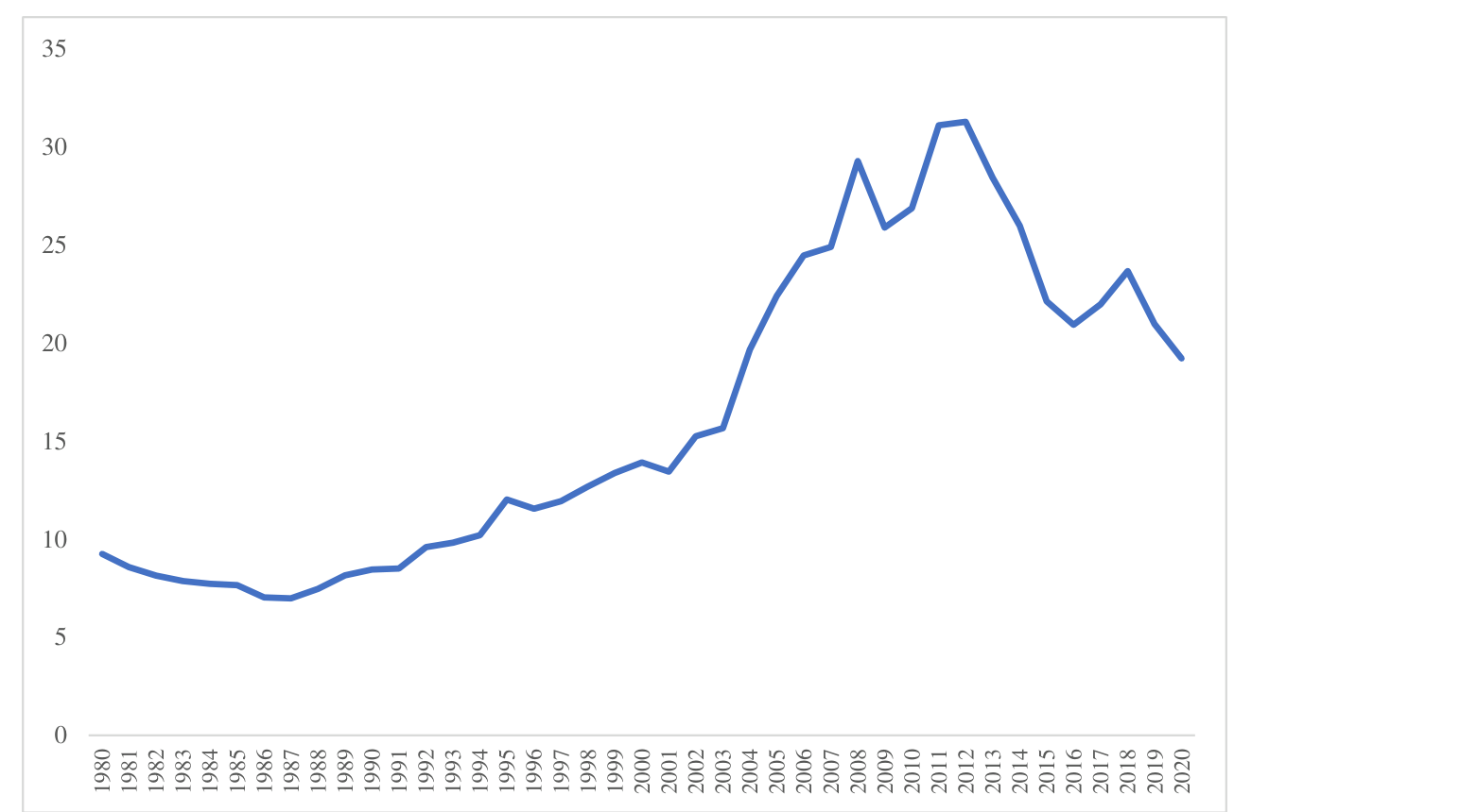
The impact of tariff on imports is discernible from visual description of the data. With tariff reforms, import-to-GDP ratio increased by about 23 percentage points between 1990 and 2012; it retreated half the distance in the period thereafter with the reversal of tariff reforms (Fig 4). The impact is empirically estimated with the help of an extended import demand equation with two additional explanatory variables, viz., SAMT and ADPINI.
The conventional aggregate import demand function takes the following form:

An alternative formulation is:

Equation-1 says that the volume of imports (M) depends on the price of imports (PM), price of domestic goods (PY), and country’s income (Y). Equation-2 relates import volume to the relative price of imports (PM/PY) and real income. Equation-2 or some variant of it is mostly used by researchers. The use of real income variable assumes the absence of ‘money illusion’ by consumer (Leamer and Stern, 2006). The relative price variable keeps the number of price terms small for estimation purposes while “still capturing the dominant sources of demand or supply substitution” (Goldstein and Khan, 1985).
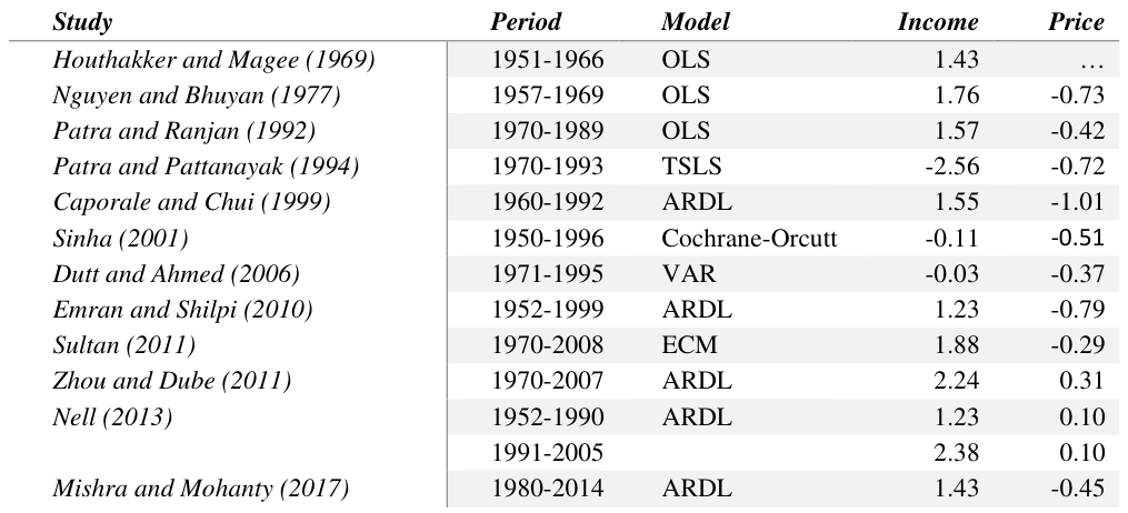
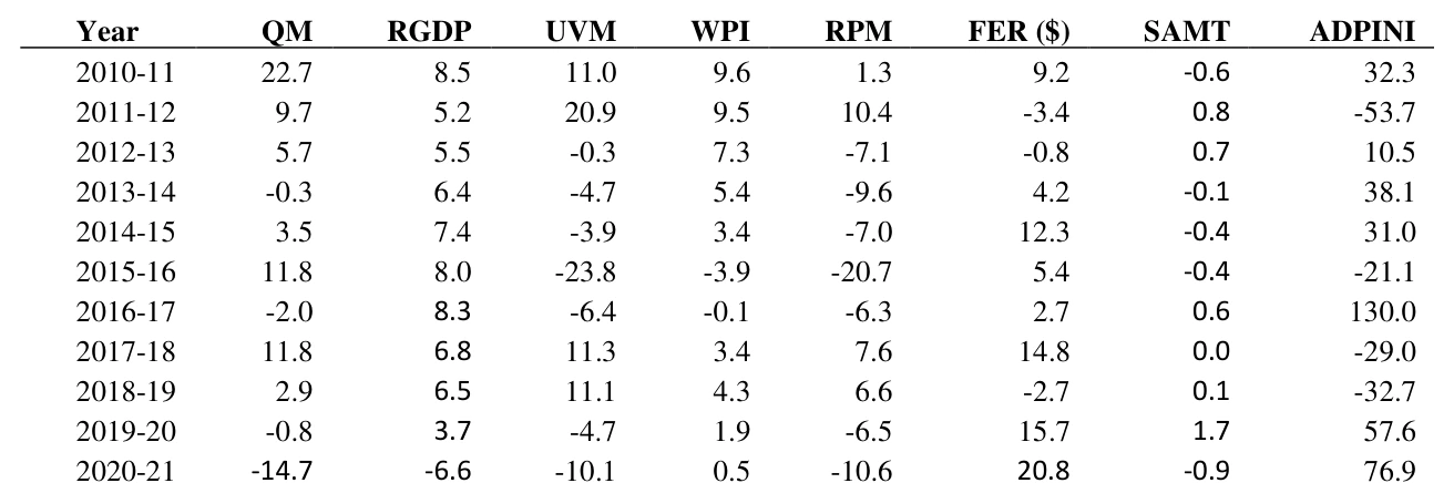
Income elasticity of India’s imports in past studies is generally more than unity, and the average of price elasticity works out to -0.4 (Table 2). Do they explain the data for recent years? Import volume declined in 2013-14, 2016-17 and 2019-20. The previous occasion when such a thing happened was in 1991-92. That was due to severe “import compression” measures dealing with the balance of payment crisis, and low economic growth. The decline in import volume in normal years occurring with the growth in real GDP and fall in relative price of imports turn the demand theory upside down (Table 3).
Some studies use foreign exchange reserves as an additional regressor. This was appropriate when imports were rationed according to policy priorities and the reserves served as a budget constraint. That is not the position now. India’s foreign exchange reserves increased during the years that had decline in import volume. This variable does not illuminate. It is here ADPINI and SAMT come into picture. Changes in SAMT and/or ADPINI coincided with most of the large variations in imports in recent years. One would think that the fall in import volume in 2020-21 was due to the pandemic. GDP declined 6.6% in 2020-21; the fall in import volume was steeper (-14.7%). Part of the explanation lies in the 77% surge in ADPINI (Table 3).
Trade policy related variables are used in import demand functions deploying ARDL models. Hoque and Yusop (2010) use import duty rate and a dummy variable representing non-tariff barriers in the import equation for Bangladesh. Dummy variable on trade liberalisation is used by Khan et al (2014) for Pakistan. In the Indian context, it should be possible to do the estimation using the data available. The number of other NTMs initiated/notified by India (countervailing duties, safeguards, and sanitary and phytosanitary measures) are not as many. On ADPINI, a couple of issues need to be sorted out: what should be the lag structure and which variable to use out of the three sets of numbers available: measures initiated, measures implemented (after investigation), and cumulated measures in force.
Anti-dumping measures are “trade remedial measures” and not “protective measures” (GoI, undated). “The purpose of anti-dumping duties is to give producers temporarily injured by highly competitive imports space to do necessary repair… But when producers keep claiming injury for two decades, it is a sure sign of fundamental inefficiency and not temporary injury” (Panagariya, 2023). In any case, the anti-dumping actions serve the purpose of curbing the imports needed by the downstream industries. India’s share in the total number of ADPINI by all countries was 27% in 2020, up from 3% in 1994. The number of measures implemented by India (e.g., 19 in 2019) is less than the measures initiated (52 in 2019). In terms of cumulated number of measures (as of 2018), India (275) was second to the USA (359). Out of the three sets of numbers, ‘measures initiated’ (i.e., ADPINI) is the relevant variable for import demand function. The timeline prescribed for investigation of anti-dumping cases would be useful in deciding the lag structure. Excerpts from a booklet (GoI, undated) are below:
“Anti-dumping investigations are generally initiated after examination of merits of the case, within 30 days of acceptance of an application (p.8). A provisional duty not exceeding the margin of dumping or injury, whichever is less, may be imposed by the Central Government based on the preliminary finding recorded by the Authority. The provisional duty can be imposed only after the expiry of 60 days from the date of initiation of investigation. The provisional duty will remain in force only for a period not exceeding 6 months, extendable to 9 months under certain circumstances (p.15). Normal time allowed by the statute for conclusion of investigation and submission of final findings is one year from the date of initiation of the investigation. This may be extended up to a period of 6 months, in exceptional circumstances, by the Central Government” (p.16).
ADPINI would impact imports during the current- and subsequent year. On tariff, the substantive issue relates to its measure. Citing the low weighted average tariff and low customs collection rates, Singh (2017) argues that “the conventional view that India is a high tariff economy is incorrect”. The measures referred to by Singh can be misleading, as very little imports might take place at higher duty rates. If the value of import of a product attracting a high MFN tariff (say, 50%) is nil, it would depress the weighted average tariff. That apart, various exemptions render these measures low. Information on average MFN tariff is relevant as high tariff acts as a deterrent to import.
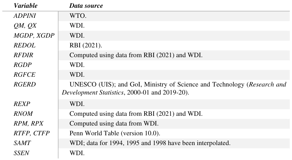
Equation 3, an extension of Equation 2 in double-log form, is the base model. Data for 1994-2020 period is used. Data sources are given in Table A.1.

Ln QM is natural log of quantity of imports of goods; ln RGDP is natural log of real GDP; Ln RPM is natural log of relative price of imports (unit value index of imports divided by domestic wholesale price index); Ln SAMT is natural log of SAMT; Ln ADPINI is natural log of number of ADPINI; and ε: error term; subscript t denotes time. The coefficient of Ln RGDP is expected to be positive in keeping with the theory of imperfect substitution that precludes import of inferior goods. The coefficient of Ln RPM would be negative in accordance with the demand theory. Demand for imported goods rises with increase in domestic prices, while increase in import price reduces the demand. Supply elasticities are assumed to be infinite. The coefficients of SAMT and ADPINI are expected to be negative.
Following Giovannetti (1989), expenditure components have been used (in place of GDP) in import function in several studies (Abbott and Seddighi, 1996; Tang, 2013; Narayan and Narayan, 2005; Agbola, 2009; Yoon and Seddighi, 2019). Giovannetti (1989) uses two components: consumption, and a composite variable named ‘investment, stock-building and exports’ (ISX). Others use more, and many country-specific findings emerge. In some studies, the coefficient of exports is large and that of investment is small (even negative). The large coefficient of exports is realistic in countries exporting manufactured products with high import content. The small/negative coefficient of investment can be due to estimation errors. In India’s case, gross fixed capital formation (GFCF) tracked the movements in steel prices (Mallik, 2019). Private final consumption expenditure (PFCE) is derived by netting out government final consumption expenditure (GFCE) and investment from the output of various products. Stock-building can at times be negative (Giovannetti, 1989), while valuables and statistical discrepancy are imponderables. Considering these aspects, this paper uses two expenditure components (exports and domestic demand), capturing the role of external- and domestic demand. Two variables – Ln RDD (natural log of real domestic demand) and Ln REXP (natural log of real exports of goods and services) – replace Ln GDP in the equations henceforth.
Equation-3 assumes that importers are always on their demand schedules such that demand equals the actual level of imports. However, imports may take time to adjust to their long run equilibrium level following a change in any of their determinants due to various factors, such as, adjustment costs, inertia, habit or lags in perceiving the changes (Carone, 1996). To capture the speed of adjustment, the following error correction model is estimated:
∆ln QMt = β0 + ∑ β1∆ ln Mt −i + n i=1 ∑ β2∆ ln RDDt − n i=0 i + ∑ β3∆ ln REXPt −i + n i=0 ∑ β4∆ ln RPMt −i + n i=0 ∑ β5∆ ln SAMTt − n i=0 i + ∑ β6∆ ln ADPINIt −i + n i=0 ψεt −1 + μt
(4)
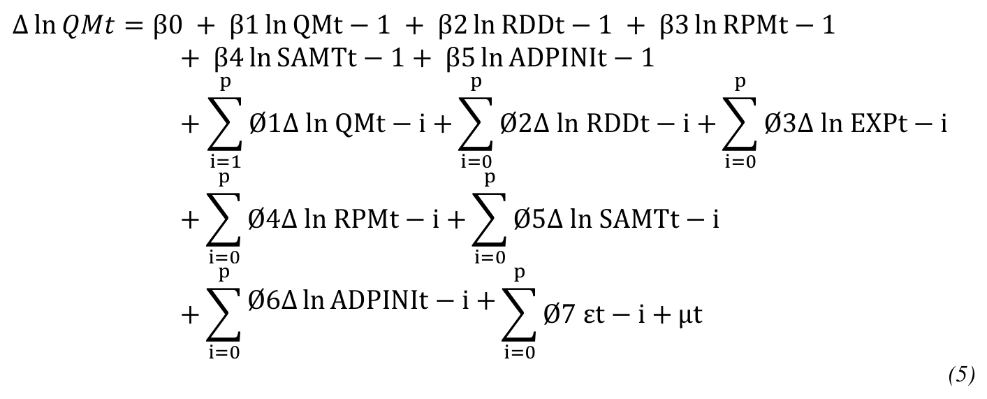
∆ represents change, and εt-1 is one period lagged error correction term (estimated from equation-3). ψ measures the speed of adjustment. Other variables are as defined earlier. The bounds testing procedure developed by Pesaran, Shin and Smith (Pesaran et al. 2001) has been used to test the cointegrating relationship in levels among the variables. For this purpose, Equation-3 was estimated as a conditional ARDL model as in Equation-5. The decision rule is the following. When the computed F statistic is higher than the upper bound of the critical values, the null hypothesis of no cointegration is rejected. When the computed F statistic is lower than the lower bound of the critical values, the null cannot be rejected. When the computed F statistic lies between the lower- and upper bounds of the critical values, it does not lead to a decision about the cointegration, and the researcher would have to check the unit roots of the variables.
3.2. Productivity Model
Productivity would depend on many factors: education, health, infrastructure, institutions, openness, competition, financial development, geographical predicaments and absorptive capacity, etc. (Isaksson, 2007). The availability and quality of the data on these things poses a problem in time series analysis. Studies on India are very few, and divergent conclusions emerge about the role of trade and foreign direct investment (FDI). Trade liberalization, among other things, had a role in the productivity surge in India around 1980 (Rodrik and Subramanian, 2005). Trade openness is cointegrated with TFP in the long-run; in the short-run, Granger causality runs from trade openness to TFP (Haider et al, 2019). Trade-induced productivity gains in Indian manufacturing largely operate through imports (Rijesh, 2019). Inward FDI improves TFP growth, while trade has a ‘detrimental’ effect (Choi and Baek, 2017). Inflation and financial development impact TFP positively; FDI, imports, and capital formation have a positive but insignificant impact while exports have a significant ‘negative’ impact (Malik et al, 2021).
Equation 6 is the base model. Data for 1980-2018 is used. The error correction form and the equation used for bounds test are not given here for brevity: they are similar as in the imports model.

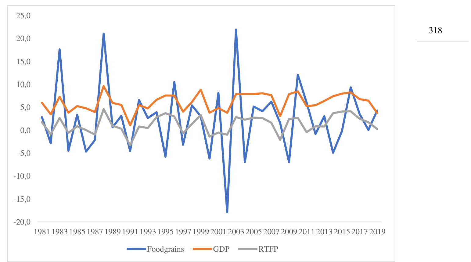
Ln RTFP is natural log of TFP at constant prices; Ln RGERD is natural log of real gross expenditure on research and development (GERD) (proxy for innovation); Ln SSEN is natural log of secondary school enrolment (% of population), gross (proxy for education); Ln MGDP is natural log of imports-to-GDP ratio (%) (proxy for competition in domestic product market); Ln XGDP is natural log of exports-to-GDP ratio (%) (proxy for scale economy); Ln RFDIR is natural log of real FDI in Rupee (proxy for access to global finance/know-how); DCRISIS is a dummy variable for crisis (takes value 1 in 1991 and 2008, zero in other years); and DSIA is a dummy variable for severely impaired agriculture (takes value 1 in 2002, zero in other years). The crises of 1991 and 2008 adversely impacted activity. In 2002, due to a severe drought, marked by a 56% below normal rainfall in the crucial sowing month of July, output of foodgrains declined by 18%, impacting GDP as well as TFP (Fig 5).
3.3. Exports Model
World income and relative price are the main determinants of exports. Elasticity estimates of recent studies vary (Table 4). The Rangarajan-Kannan paper says that nominal exchange rate is the only policy variable available for adjustment. The HLAG (op cit.) tells the opposite: “It is often (most often) contended by experts that yes, Indian exports have performed badly but it is due to our exchange rate policy… this is at best a bad (and untrue) excuse… While one view could be that devaluation of the currency could enhance exports, our analysis shows that this may not be a viable option, or an effective option.” (GoI 2019: p.xxi).

Equation 7 is the base model. Data for 1980-2019 period is used.

Ln X is natural log of volume index of India’s exports; Ln RGDPW is natural log of real GDP of the World; Ln MGDP is natural log of imports to GDP ratio (%); and Ln RTFP: natural log of real TFP. While the role of world GDP and relative price of exports is the same as in the import function, difference lies in the assumption on supply elasticity. The computed value of F statistic of the traditional export equation (with Ln RGDPW and Ln RPX as regressors) at 2.95 was lower than the lower bound of the critical values, which is no cointegration. It indicates that supply elasticities are not as infinite as one assumes. 7 Inclusion of the additional variables (Ln MGDP and Ln RTFP) makes a difference.
3.4. GDP Model
Equation 8 is the base model. Data for 1990-2019 period is used.

Ln RNOM is natural log of real non-oil imports; Ln REDOL is natural log of Rupee-Dollar exchange rate; and Ln RGFCE is natural log of real GFCE. Other variables are as defined earlier.
The literature provides divergent views on the impact of these variables. The first three are somewhat less contentious. There is evidence supporting export-led growth and import-led growth propositions in the Indian context (Mishra, 2012; and Maitra, 2020). Exchange rate has a negative impact. An increase in the exchange rate (expressed as Indian Rupees per unit of US Dollar) increases the prices of traded goods (and ultimately the general price level) that reduces the aggregate demand and slows economic growth (Maitra, 2020).
The empirical evidence on FDI varies. FDI has a small positive impact on GDP (Biswas and Shah, 2014). FDI does not significantly impact GDP (Seshaiah et al, 2018). FDI inflow is the outcome of GDP growth (Das and Das, 2020): this conclusion is based on the Granger causality tests, while the study reports a negative impact of FDI in the shortrun model.
Evidence on the relationship between GFCE and GDP is mixed. Analysis of panel data for 182 countries covering the 1950-2004 period shows strong support for both Wagner's law (the observation that public expenditure increases as national income rises) and the hypothesis that government spending is helpful to economic growth (Wu et al, 2010). In the Indian context too, government expenditure has a significant positive impact on GDP (Sheshaiah et al, 2018).
3.5. Bounds tests
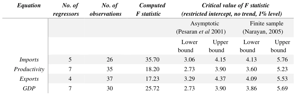
The computed value of the F statistic in all four models are higher than the upper bound of the critical values at 1% level of significance relating to large sample (Pesaran et al,
7 Reasons are many. Exports of several products originate from micro, small and medium enterprises (MSMEs), where the activity is impeded due to inadequate infrastructure, absence of formalization, lack of backward/forward linkages, lack of credit, low technology, etc. (Das, 2008 and 2017; Bhattacharya, 2013; Nair and Das, 2019). Financing constraints are a binding factor for exports (Mukherjee and Chanda, 2021). Agricultural exports suffer due to frequent changes in various non-tariff barriers (GoI 2017, 101).
- as well as finite sample (Narayan, 2005) confirming the existence of a cointegrating relationship in levels among the variables in these models (Table 5).
3.6. Diagnostics
The error correction models were put to various diagnostic tests. The LM tests sustain the null hypotheses of no autocorrelation. The Breusch-Pagan-Godfrey tests retain the null hypotheses of no heteroskedasticity. The models pass the Jarque Bera normality test. The Ramsey RESET tests show that the models are correctly specified. The cumulative sum of recursive residuals (CUSUM) and CUSUM square plots (Fig 16-19) do not show instability. The coefficients of error correction terms are negative and significant. Convergence is rapid but oscillatory in the imports model (118% of adjustment takes place within a year), while in productivity, exports and GDP models, 44%, 40% and 54%, respectively, of the correction take place within a year. The adjusted R-squares explain 94%, 86%, 90% and 92% of the variation in imports, productivity, exports and GDP models, respectively (Table 7, 9, 11 & 14).
4. Results and Discussions
The coefficients of all the determinants of imports (both in the long- and short-run models) are statistically significant with the expected sign. A 1% increase in exports increases imports by 0.35%, while a 1% increase in domestic demand increases imports by 0.32%. These are smaller than the income elasticity estimates of past studies, while the price elasticity (-0.34) is comparable. A 1% increase in SAMT decreases imports by 0.82%, while a 1% increase in ADPINI decreases imports by 0.07% (Table 6 & 7).
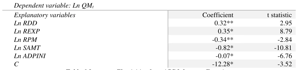
Accessible table text
| — | Dependent variable: Ln QM t | — | — | — | — | — | — | — |
|---|---|---|---|---|---|---|---|---|
| — | Explanatory variables | — | — | Coefficient | — | — | t statistic | — |
| — | Ln RDD | — | 0.32** 2.95 | — | — | — | — | — |
| — | Ln REXP | — | — | 0.35* | — | — | 8.79 | — |
| — | Ln RPM | — | -0.34** -2.84 | — | — | — | — | — |
| — | Ln SAMT | — | — | -0.82* | — | — | -10.81 | — |
| — | Ln ADPINI | — | -0.07* -6.76 | — | — | — | — | — |
| — | C | — | — | -12.28* | — | — | -3.52 | — |
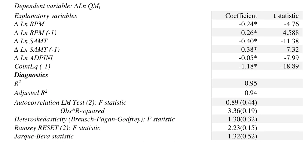
Accessible table text
| — | Dependent variable: ∆Ln QM t | — | — | — | — | — | — | — |
|---|---|---|---|---|---|---|---|---|
| — | Explanatory variables | — | — | Coefficient | — | — | t statistic | — |
| — | ∆ Ln RPM | — | -0.24* -4.76 | — | — | — | — | — |
| — | ∆ Ln RPM (-1) | — | — | 0.26* | — | — | 4.588 | — |
| — | ∆ Ln SAMT | — | -0.40* -11.38 | — | — | — | — | — |
| — | ∆ Ln SAMT (-1) | — | — | 0.38* | — | — | 7.32 | — |
| — | ∆ Ln ADPINI | — | -0.05* -7.99 | — | — | — | — | — |
| — | CointEq (-1) | — | — | -1.18* | — | — | -18.89 | — |
| — | Diagnostics | — | — | — | — | — | — | — |
| — | R2 | — | — | 0.95 | — | — | — | — |
| — | Adjusted R2 | — | 0.94 | — | — | — | — | — |
| — | Autocorrelation LM Test (2): F statistic | — | — | 0.89 (0.44) | — | — | — | — |
| — | Obs*R-squared | — | 3.36(0.19) | — | — | — | — | — |
| — | Heteroskedasticity (Breusch-Pagan-Godfrey): F statistic | — | — | 1.30(0.32) | — | — | — | — |
| — | Ramsey RESET (2): F statistic | — | 2.23(0.15) | — | — | — | — | — |
| — | Jarque-Bera statistic | — | — | 1.32(0.52) | — | — | — | — |
SSEN, RGERD and XGDP have a positive impact on productivity in the long run. MGDP has a negative impact, suggesting efficiency loss in the import-competing industries. However, import-induced productivity gains captured in the short-run model are immense: the coefficients of current- and past changes in MGDP are positive and significant. The position of FDI is similar: its current change has a negative impact, 1year lag is insignificant, and 2-year lag has a significant positive impact (Table 8 & 9). FDI data was derived by converting US Dollar-denominated FDI flows into Indian Rupee and deflating by the GDP deflator, making it comparable with the dependent variable. Even then, any strong conclusion about the role of FDI is best avoided, given the data weaknesses (Rao and Dhar, 2018).
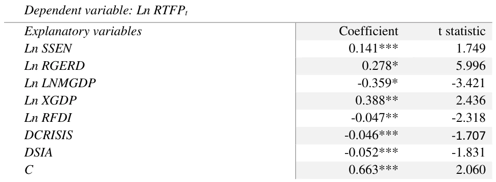
Accessible table text
| Dependent variable: Ln RTFP t | — | — | — | — | — | — | — | — |
|---|---|---|---|---|---|---|---|---|
| — | Explanatory variables | — | — | Coefficient | — | — | t statistic | — |
| — | Ln SSEN | — | 0.141*** 1.749 | — | — | — | — | — |
| — | Ln RGERD | — | — | 0.278* | — | — | 5.996 | — |
| — | Ln LNMGDP | — | -0.359* -3.421 | — | — | — | — | — |
| — | Ln XGDP | — | — | 0.388** | — | — | 2.436 | — |
| — | Ln RFDI | — | -0.047** -2.318 | — | — | — | — | — |
| — | DCRISIS | — | — | -0.046*** | — | — | -1.707 | — |
| — | DSIA | — | -0.052*** -1.831 | — | — | — | — | — |
| — | C | — | — | 0.663*** | — | — | 2.060 | — |
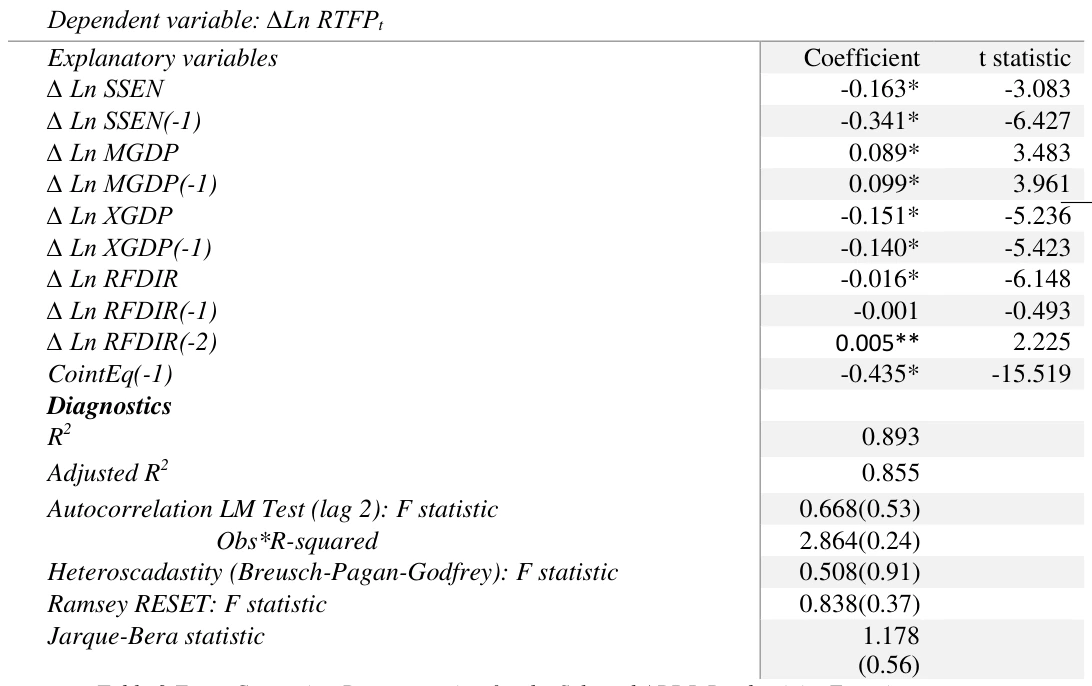
Accessible table text
| Dependent variable: ∆Ln RTFP t | — | — | — | — | — | — | — | — | — |
|---|---|---|---|---|---|---|---|---|---|
| — | Explanatory variables | — | — | Coefficient | — | — | t statistic | — | — |
| — | ∆ Ln SSEN | — | — | — | — | — | — | — | — |
| — | ∆ Ln SSEN(-1) | — | — | -0.341* | — | — | -6.427 | — | — |
| — | ∆ Ln MGDP | — | — | — | — | — | — | — | — |
| — | ∆ Ln MGDP(-1) | — | — | 0.099* | — | — | 3.9 | 61 | — |
| — | ∆ Ln XGDP | — | — | — | — | — | — | — | — |
| — | ∆ Ln XGDP(-1) | — | — | -0.140* | — | — | -5.423 | — | — |
| — | ∆ Ln RFDIR | — | — | — | — | — | — | — | — |
| — | ∆ Ln RFDIR(-1) | — | — | -0.001 | — | — | -0.493 | — | — |
| — | ∆ Ln RFDIR(-2) | — | — | — | — | — | — | — | — |
| — | CointEq(-1) | — | — | -0.435* | — | — | -15.519 | — | — |
| — | Diagnostics | — | — | — | — | — | — | — | — |
| — | R2 | — | — | 0.893 | — | — | — | — | — |
| — | Adjusted R2 | — | — | — | — | — | — | — | — |
| — | Autocorrelation LM Test (lag 2): F statistic | — | — | 0.668(0.53) | — | — | — | — | — |
| — | Obs*R-squared | — | — | — | — | — | — | — | — |
| — | Heteroscadastity (Breusch-Pagan-Godfrey): F statistic | — | — | 0.508(0.91) | — | — | — | — | — |
| — | Ramsey RESET: F statistic | — | — | — | — | — | — | — | — |
| Jarque-Bera statistic | Jarque-Bera statistic | — | — | 1.178 | — | — | — | — | — |
| — | — | — | — | (0.56) | — | — | — | — | — |
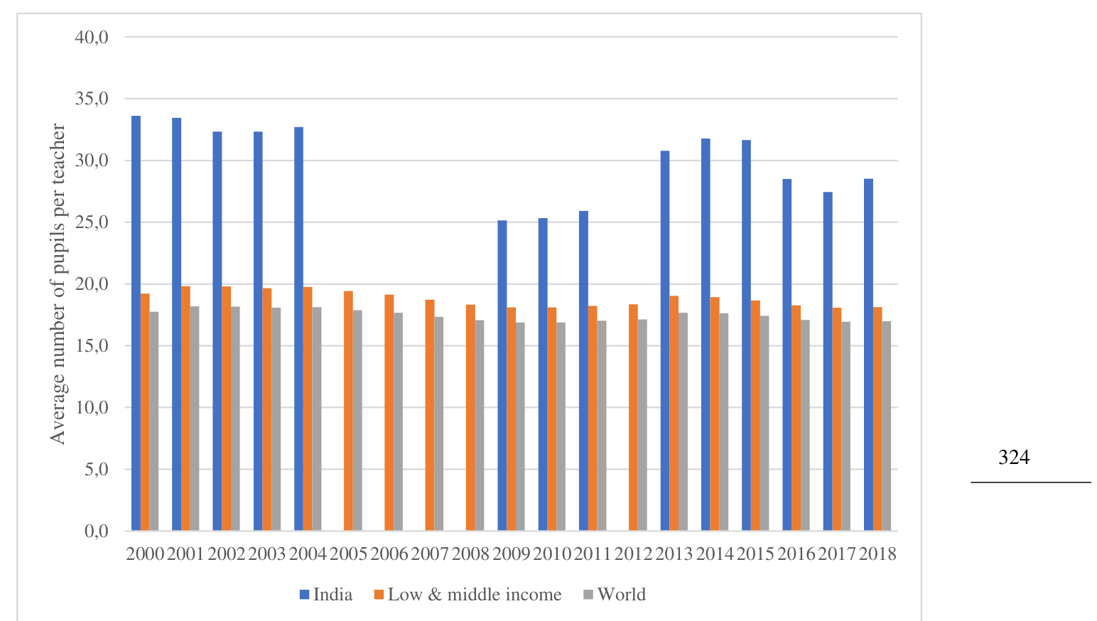
The short-run negative impact of SSEN on TFP may be a reflection of the shortages of teachers. The pupil-teacher ratio (PTR) in India’s secondary/senior secondary schools
(between 43:1 and 47:1 in 2018-19, according to UNESCO, 2021) was far greater than in LMY country-group (secondary: 18.1:1; upper secondary: 18.6:1). The PTR in India fluctuated (Fig 6). A study on TFP in Pakistan reports negative coefficients of government expenditure on education both in long- and short-run, while the coefficient of secondary enrolment ratio is negative in the long-run but positive in the short-run (Adnan et al, 2020).
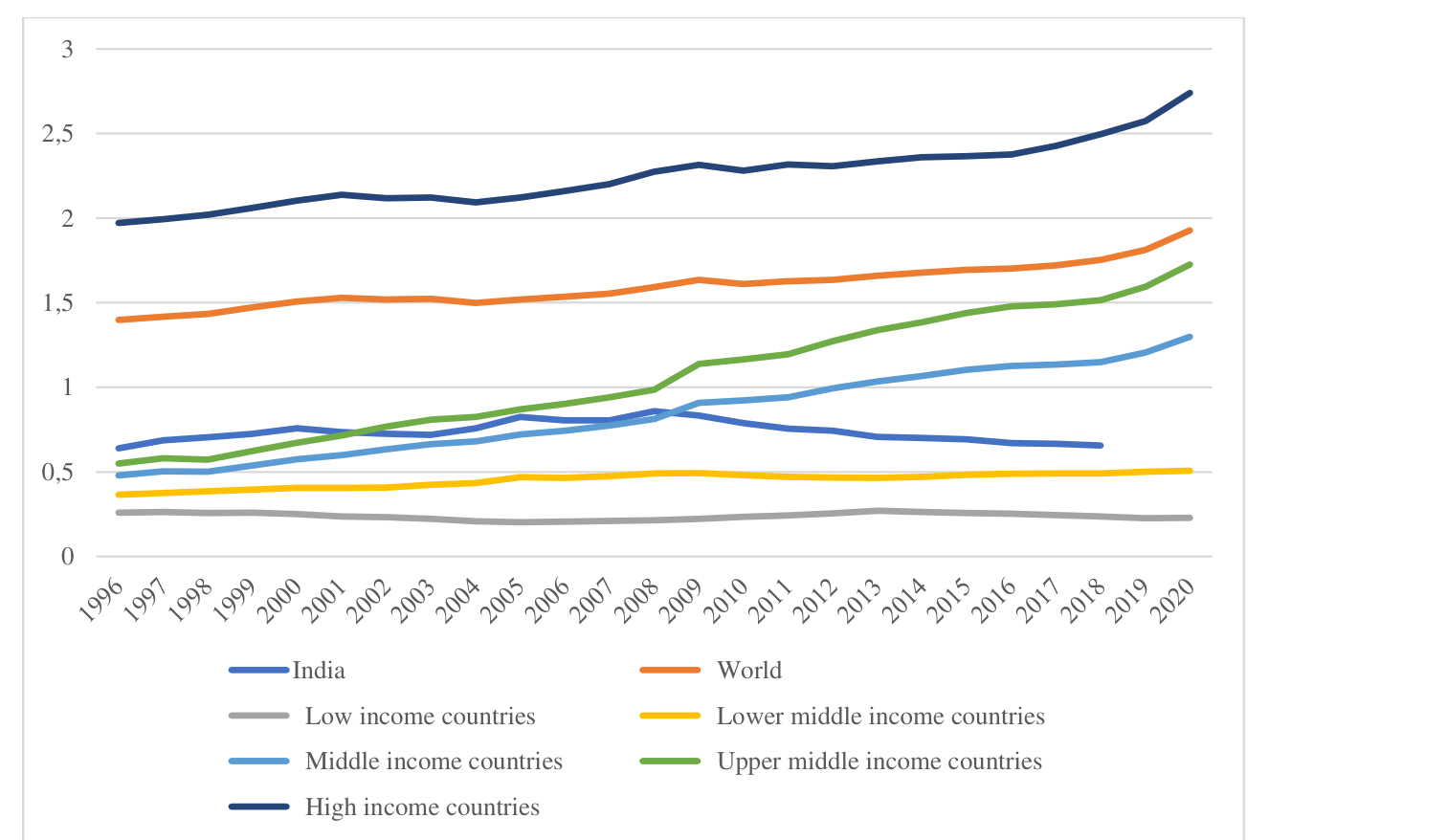
The crucial long-run determinants of productivity (SSEN and RGERD) faltered after 2008 (Fig 7). During the 1990s, India’s R&D spending (% of GDP) was higher than the averages of middle-income country groups; the increase in India’s R&D spending observed during 2000-2008 was broadly comparable; the decline after 2008 was a deviant trend (Fig 8).
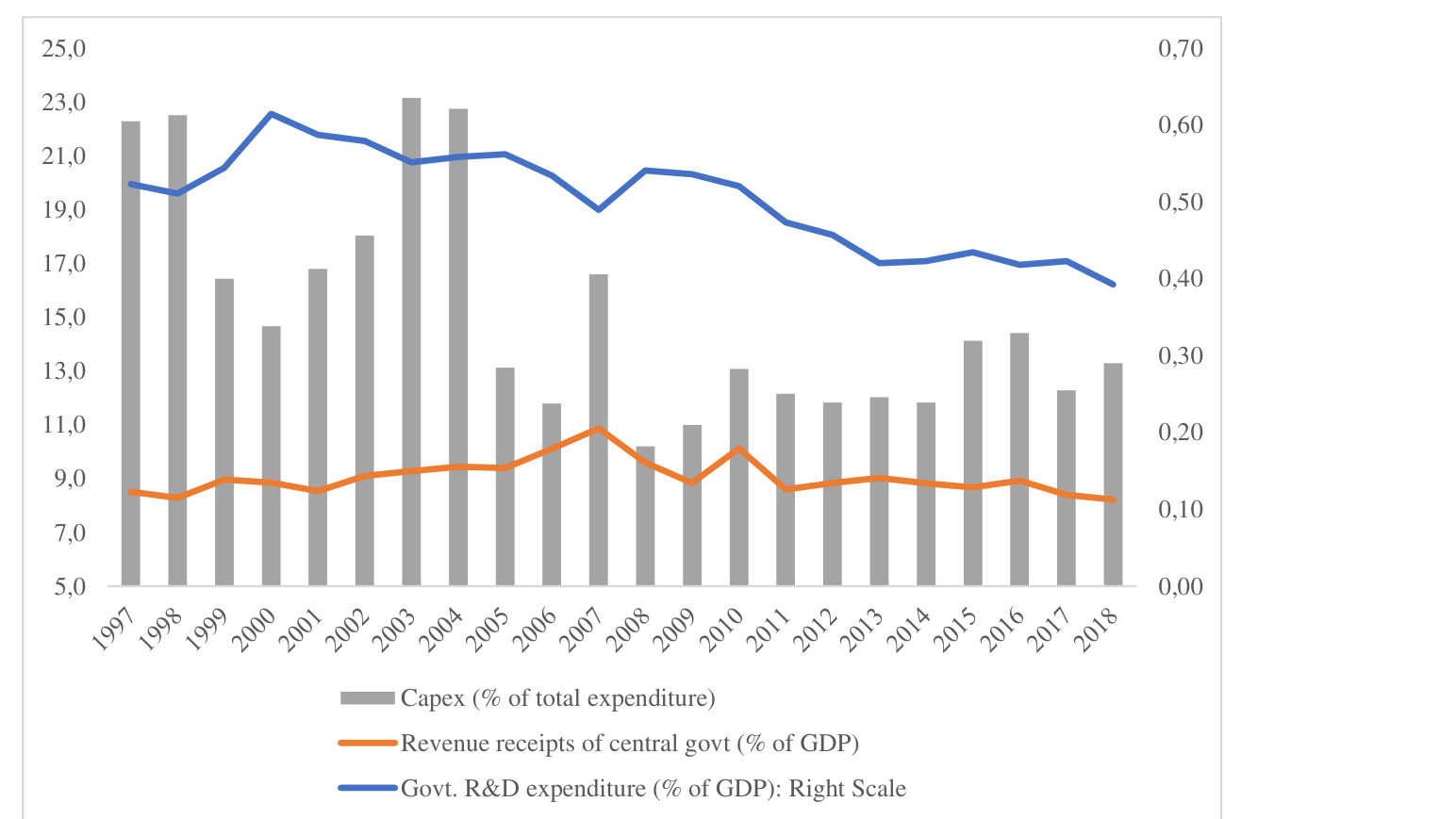
Governments contribute about 60% of GERD in India, unlike other major economies where most of it is done by the business. Government R&D (% of GDP) fell regularly during 2000-2018 while business R&D, which had grown from 0.14% of GDP in 2000 to 0.32% in 2008, fell to 0.26% in 2018.
Government R&D would depend on their revenues and priorities. The priority in Union budgets these days is on CAPEX. The CAPEX of the central Government is budgeted to grow by 37.5% at current prices in 2023-24, on top of 30.9% (on average) during 2021- 23,8 as the revenue expenditure grows by only 1.2% in 2023-24, over 5.9% during 2021-23 that fell short of the inflation.9 During the 1997-2018 period, central government’s revenue receipts rarely exceeded 10% of GDP and the proportion was declining; within this budget constraint, the CAPEX push years were witness to a dip in governments’ R&D spending (Fig 9).

8 Include revised estimates for 2022-23. 9 GDP deflator recorded an increase of 8.4% during 2021-23.
Business R&D would be related to government policy. There is an inverse relationship between tariffs and business R&D with a correlation coefficient of -0.91 (Fig 10), reinforced by the activity-wise data (Fig. 11). If the tariffs were revenue-raising (Panagariya, 2022b) and it is assumed that the elevated tariff reduces the incentive for innovation by firms operating in a relatively sheltered market, tariff reduction may improve the business R&D. If, however, the firms, unable or unwilling to spend in R&D, had lobbied for higher tariff, the policy option may be different. While this needs to be probed, a tentative policy implication may be that the private sector would hopefully increase its R&D, matching business’ in other major economies, if policies require it to operate in a competitive market, not a sheltered market.


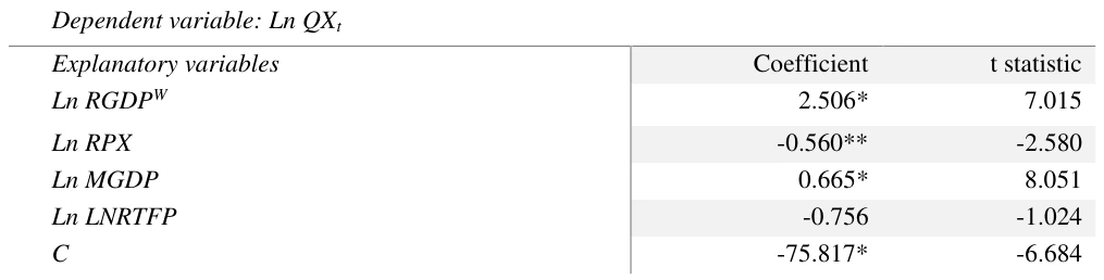
In the long-run exports model, a 1% increase in world GDP increases India’s exports by 2.5%, a 1% increase in RPX decreases exports by 0.6%, and a 1% increase in MGDP increases exports by 0.7%. In the short run, the contemporaneous change in world GDP has a positive impact, RPX has a negative impact, and past change of TFP has a positive impact (Table 10 & 11).
Accessible table text
| Dependent variable: Ln QX t | ent variable: Ln QX t | — | — | — | — |
|---|---|---|---|---|---|
| Explan | atory variables | Coefficient | — | t statistic | — |
| Ln RGDPW | DPW | 2.506* 7.015 | — | — | — |
| Ln RPX | — | -0.560** | — | -2.580 | — |
| Ln MG | DP | 0.665* 8.051 | — | — | — |
| Ln LNR | TFP | -0.756 | — | -1.024 | — |
| C | — | -75.817* -6.684 | — | — | — |

Accessible table text
| Dependent variable: ∆Ln QX t | — | — | — | — | — | — | — | — |
|---|---|---|---|---|---|---|---|---|
| — | Explanatory variables | — | — | Coefficient | — | — | t statistic | — |
| ∆ Ln RGDPW | ∆ Ln RGDPW | — | 2.010* 4.958 | — | — | — | — | — |
| ∆ Ln RGDPW(-1) | — | — | -1.584* | — | — | -3.945 | — | — |
| ∆ Ln RGDPW(-2) | — | — | -1.198* -3.355 | — | — | — | — | — |
| — | ∆ Ln RPX | — | — | -0.765* | — | — | -9.455 | — |
| — | ∆ Ln RTFP | — | -0.385 -0.135 | — | — | — | — | — |
| — | ∆ Ln RTFP(-1) | — | — | 1.012* | — | — | 3.583 | — |
| — | CointEq(-1) | — | -0.406* -11.139 | — | — | — | — | — |
| — | Diagnostics | — | — | — | — | — | — | — |
| R2 | R2 | — | 0.914 | — | — | — | — | — |
| Adjusted R2 | — | — | 0.897 | — | — | — | — | — |
| — | Autocorrelation LM Test (lag 2): F statistic | — | 1.090(0.35) | — | — | — | — | — |
| — | Obs*R-squared | — | — | 3.20(0.20) | — | — | — | — |
| — | Heteroscadastity (Breusch-Pagan-Godfrey): F statistic | — | 0.345(0.97) | — | — | — | — | — |
| — | Ramsey RESET: F statistic | — | — | 3.992(0.057) | — | — | — | — |
| — | Jarque-Bera statistic | — | 1.596(0.450) | — | — | — | — | — |
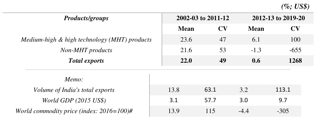
As explained, the reduction in innovation efforts hurt exports via productivity. The role of technology can also be gauged from the commodity-wise data: exports of mediumhigh and high technology (MHT) products grew during 2012-20 and the changes were relatively stable; exports of non-MHT products declined and the changes were volatile reflecting the movements in commodity prices (Table 12).
It is often argued that the recent slow growth of India’s exports was due to the slowdown in global economy. The 3% growth of world GDP during 2012-2019 was only marginally lower than the growth recorded during 2002-2011, and this will explain very little of the observed reduction in the growth rate of India’s exports (Table 12). The drop in India’s export growth can possibly be attributed to the de-globalization. While it is difficult to be quantified in the time series framework, some evidence from cross-country data is presented in Section 5.
(%; US$)
Medium-high & high technology (MHT) products 23.6 47 6.1 100
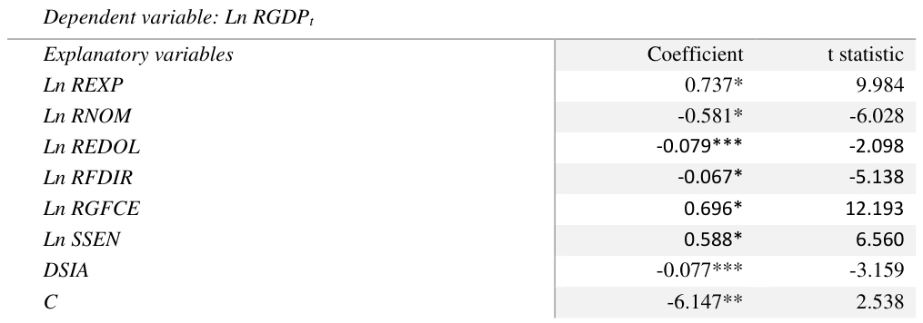
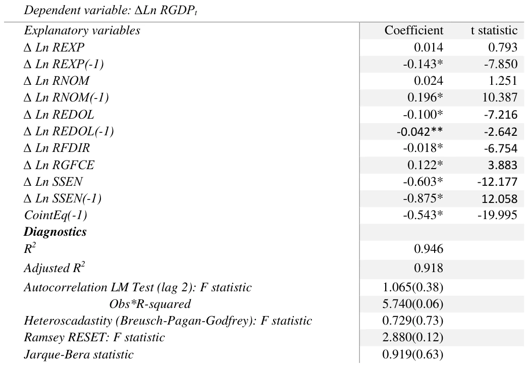
Exports, GFCE and SSEN positively impact GDP in the long run, while non-oil imports, exchange rate and FDI impact it negatively. The cautionary remark on FDI made earlier applies here as well. In the short-run, exports, non-oil imports and GFCE have a positive impact, while SSEN has a negative impact, consistent with the evidence from the productivity model (Table 13 & 14). The positive impact of GFCE on GDP is another reason, besides the fall in Government R&D expenditure in the CAPEX push years, why CAPEX push at the cost of essential current expenses may be a misplaced priority.
Accessible table text
| Dependent variable: Ln RGDP t | — | — | — | — | — | — | — | — |
|---|---|---|---|---|---|---|---|---|
| — | Explanatory variables | — | — | Coefficient | — | — | t statistic | — |
| — | Ln REXP | — | 0.737* 9.984 | — | — | — | — | — |
| — | Ln RNOM | — | — | -0.581* | — | — | -6.028 | — |
| — | Ln REDOL | — | -0.079*** -2.098 | — | — | — | — | — |
| — | Ln RFDIR | — | — | -0.067* | — | — | -5.138 | — |
| — | Ln RGFCE | — | 0.696* 12.193 | — | — | — | — | — |
| — | Ln SSEN | — | — | 0.588* | — | — | 6.560 | — |
| — | DSIA | — | -0.077*** -3.159 | — | — | — | — | — |
| — | C | — | — | -6.147** | — | — | 2.538 | — |
The recent economic slowdown was due to the subdued productivity and weak exports. The ‘extra slow’ growth of 2019-20 (3.9% vis-a-vis 7% during 2012-19, on average) reflected the absence of TFP growth,10 aggravated by the deceleration in the growth rate of GFCE (to 3.4% from 6.7% in 2018-19) and the sharp decline in non-oil imports (-8.3%) partly attributable to the ‘extra fast’ increase in SAMT and ADPINI (Table 3).
10 TFP grew by 0.1% in 2019-20 taking data from Penn World Table (version 10.01). In the Capital, Labor, Energy, Material, Services (KLEMS) framework (https://rbi.org.in/Scripts/BS_ViewPublicationReport.aspx), the TFP in Indian economy declined (-2.1%) in 2019-20, with a steep fall in manufacturing TFP (-8%). In KLEMS database for 1981-2020 period, decline in manufacturing TFP in excess of 5% occurred in two earlier years (-8.3% in 1991-92 and -12% in 1997-98). Manufacturing value added contracted during all three years (-1.2% in 1991-92, -2.9% in 1997-97 and -2.7% in 2019-20). The earlier episodes had an external dimension: deterioration in India’s balance of payment situation after the ‘Gulf crisis’ forcing the adoption of severe import compression measures (1991-92) and the slowdown in the East Asian and global economies in the wake of the ‘Asian crisis’ jolting India’s exports (1997-98) (RBI, 1992; Sathe, 1998; Berg, 1999). The 2019-20 episode was not triggered by any external crisis.
Accessible table text
| Dependent variable: ∆Ln RGDP t | — | — | — | — | — | — | — | — |
|---|---|---|---|---|---|---|---|---|
| — | Explanatory variables | — | — | Coefficient | — | — | t statistic | — |
| — | ∆ Ln REXP | — | 0.014 0.793 | — | — | — | — | — |
| — | ∆ Ln REXP(-1) | — | — | -0.143* | — | — | -7.850 | — |
| — | ∆ Ln RNOM | — | 0.024 1.251 | — | — | — | — | — |
| — | ∆ Ln RNOM(-1) | — | — | 0.196* | — | — | 10.387 | — |
| — | ∆ Ln REDOL | — | -0.100* -7.216 | — | — | — | — | — |
| — | ∆ Ln REDOL(-1) | — | — | -0.042** | — | — | -2.642 | — |
| — | ∆ Ln RFDIR | — | -0.018* -6.754 | — | — | — | — | — |
| — | ∆ Ln RGFCE | — | — | 0.122* | — | — | 3.883 | — |
| — | ∆ Ln SSEN | — | -0.603* -12.177 | — | — | — | — | — |
| — | ∆ Ln SSEN(-1) | — | — | -0.875* | — | — | 12.058 | — |
| — | CointEq(-1) | — | -0.543* -19.995 | — | — | — | — | — |
| — | Diagnostics | — | — | — | — | — | — | — |
| R2 | R2 | — | 0.946 | — | — | — | — | — |
| Adjusted R2 | — | — | 0.918 | — | — | — | — | — |
| — | Autocorrelation LM Test (lag 2): F statistic | — | 1.065(0.38) | — | — | — | — | — |
| — | Obs*R-squared | — | — | 5.740(0.06) | — | — | — | — |
| — | Heteroscadastity (Breusch-Pagan-Godfrey): F statistic | — | 0.729(0.73) | — | — | — | — | — |
| — | Ramsey RESET: F statistic | — | — | 2.880(0.12) | — | — | — | — |
| — | Jarque-Bera statistic | — | 0.919(0.63) | — | — | — | — | — |
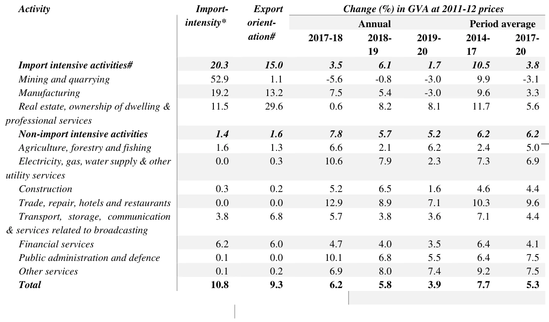
Sectoral data neatly show the role of import curbs. The average growth of 3.8% during 2017-20 in import-intensive activities was about a third of the rate recorded during 2014-17. The growth of 6.2% during 2017-20 in the non-import intensive segment was as rapid as the growth in the preceding three years. In 2019-20, import-intensive activities grew by just 1.7%. Growth moderated in the non-import intensive segment due to likely transmission of the impact of import curbs via sectoral linkages or other factors as explained econometrically (Table 15).
4.1. Results of Pair-wise Granger Causality Tests
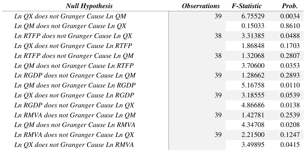
There is a unidirectional Granger causality running from exports to imports, reinforcing the evidence from the imports model. Causality runs from productivity to exports, consistent with the evidence from the short-run exports model. Causality runs from GDP to exports, 11 from imports to productivity, from imports to GDP, from imports to manufacturing value added (MVA) and from exports to MVA (Table 16). The last two and the sectoral data partly explain the poor show of manufacturing: it suffered more due to import curbs on the supply side and weak exports on the demand side, its trade exposure being relatively greater (Table 15 &16).
11 This is consistent with the view that “India’s export performance has always been greatly influenced by domestic economic factors and the performance of the domestic economy” (Nayyar, 1997, 354) and the argument made in this paper that the erosion in crucial determinants of productivity hurt India’s recent export performance.
Accessible table text
| — | Null Hypothesis | — | — | Observations | — | — | F-Statistic | — | — | Prob. | — |
|---|---|---|---|---|---|---|---|---|---|---|---|
| — | Ln QX does not Granger Cause Ln QM | — | 39 | 39 | — | — | 6.75529 | — | — | 0.0034 | — |
| — | Ln QM does not Granger Cause Ln QX | — | — | — | — | 0.15033 0.8610 | — | — | — | — | — |
| — | Ln RTFP does not Granger Cause Ln QX | — | 38 | — | — | — | 3.31385 | — | — | 0.0488 | — |
| — | Ln QX does not Granger Cause Ln RTFP | — | — | — | — | 1.86848 0.1703 | — | — | — | — | — |
| — | Ln RTFP does not Granger Cause Ln QM | — | 38 | — | — | — | 1.32068 | — | — | 0.2807 | — |
| — | Ln QM does not Granger Cause Ln RTFP | — | — | — | — | 3.70600 0.0353 | — | — | — | — | — |
| — | Ln RGDP does not Granger Cause Ln QM | — | 39 | — | — | — | 1.28662 | — | — | 0.2893 | — |
| — | Ln QM does not Granger Cause Ln RGDP | — | — | — | — | 5.16758 0.0110 | — | — | — | — | — |
| — | Ln QX does not Granger Cause Ln RGDP | — | 39 | — | — | — | 3.18555 | — | — | 0.0539 | — |
| — | Ln RGDP does not Granger Cause Ln QX | — | — | — | — | 4.86686 0.0138 | — | — | — | — | — |
| — | Ln RMVA does not Granger Cause Ln QM | — | 39 | — | — | — | 1.42781 | — | — | 0.2539 | — |
| — | Ln QM does not Granger Cause Ln RMVA | — | — | — | — | 4.34708 0.0208 | — | — | — | — | — |
| — | Ln RMVA does not Granger Cause Ln QX | — | 39 | — | — | — | 2.21500 | — | — | 0.1247 | — |
| — | Ln QX does not Granger Cause Ln RMVA | — | — | — | — | 3.49895 0.0415 | — | — | — | — | — |
5. Why Doesn’t Government Support Improve the Fortunes of Manufacturing?
At present, PLI is the main form of government support to manufacturing. Several issues, such as, the higher price of PLI-enabled domestically produced goods (e.g., mobile phones), likely adverse impact on exports of user industries if the PLI-supported products (e.g., semiconductors) do not become globally cost-competitive, and continuation of production (after PLI), etc. have been raised (Rajan and Chauhan, 2022). It’s a method of monetising the productivity deficit: “if we are 30% less productive than China, then the government will, through PLI, monetise that productivity deficit for the private sector, provided the latter invests in large global-scale capacities” (Mukherjee, 2022). The PLI for large scale electronics announced in April 2020 – cognizant of the sector’s disability of around 8.5% to 11% vis-à-vis competing nations (due to lack of adequate infrastructure, domestic supply chain and logistics, high cost of finance, inadequate availability of quality power, limited design capabilities and focus on R&D by the industry, and inadequacies in skill development) – provides a subsidy of 4% to 6% on incremental sales for a period of five years (https://www.meity.gov.in/esdm/pli). The scheme for semiconductors provides a fiscal support of 50% of the project cost.
5.1. On subsidizing the productivity gap
At the macro level, the relative productivity in India (about 44% of USA in 2019, according to Penn World Table) is comparable with China, Indonesia and Thailand, but lower than that of Malaysia, Philippines and Sri Lanka (Fig 12). WDI data show that the share of MVA in GDP fell between 2010 and 2019 in all these countries, regardless of the level or the trend in relative productivity: China (-4.8 percentage points (pp)), India (-3.6 pp), Indonesia (-2.3 pp), Malaysia (-2 pp), Philippines (-3.4 pp), Sri Lanka (-2.3 pp), and Thailand (-5.3 pp). Across regions, the GDP share of MVA fell in South Asia (-2.5 pp), East Asia and Pacific (-1.1 pp), and North America (-0.8 pp), contrasting the increases in Latin America and Caribbean (1.2 pp), sub-Saharan Africa (1.2 pp), and EU (0.4 pp).

It appears that manufacturing in Asia and North America was severely impacted by the de-globalization, the protectionism being more acute in these regions. Information on tariffs and NTM is available, although de-globalization is a larger concept and the quantification of its impact is difficult. Tariff is high in South Asia (12.3% in 2017); it’s a mixed bag in East Asia and Pacific (tariff is very low in Hong Kong, Singapore and Australia, but relatively high in South Korea, Viet Nam and Indonesia); and is low in North America. Tariff also varies in the regions that had improvement in the relative performance of manufacturing: 5.1% in EU, but roughly twice that level in the other two regions. It is the NTM that provides the dividing line. Its use is high in Asia and North America and relatively low in Latin America and Caribbean, sub-Saharan Africa, and EU. In fact, seven out of world’s top 15 users of NTM are countries in Asia Pacific: China (1st), Thailand (3rd), India (4th), Philippines (5th), Korea (7th), Japan (9th) and Australia (10th). Three of the major North American countries also feature in the list: USA (2nd), Canada (13th) and Mexico (15th) (Thompson, 2021).
5.2. Evidence from Two Manufacturing Industries
5.2.1. Mobile Phones
Support to domestic manufacturing of mobile phones under the “Make in India” initiative begun with a differential excise duty dispensation announced in Union Budget, 2015-16 that included a countervailing duty (CVD) of 12.5% on imports and excise duty of 1% without input tax credit or 12.5% with input tax credit. Budget 2016-17 withdrew the exemption from basic customs duty (BCD)/CVD)/special additional duty (SAD) on charger/ adapter, battery and wired headsets/speakers used for manufacture of mobile phone, and applied BCD/CVD of 12.5% and SAD of 4%. Budget 2018-19 hiked customs duties on mobile phones from 15% to 20% and on its accessories from 7.5%-10% to 15%. Budget 2020-21 raised customs duty on printed circuit board assembly (PCBA) of mobile phones from 10% to 20%. A ‘Phased Manufacturing Programme (PMP) to promote indigenous manufacturing of cellular mobile handsets, its sub-assemblies and parts/subparts/inputs of the sub-assemblies thereof’ through “appropriate fiscal and financial incentives” was announced in April 2017. This was followed by a PLI scheme for electronics manufacturing (applicable for mobile phones and specified electronic components) announced in April 2020, later extended to other products.
Exports of mobile phones (HS: 851712), which remained subdued during 2013-18, improved from 2018-19 presumably due to the PMP/PLI (Fig 13). However, data from Annual Survey of Industries on manufacture of communication equipment (NIC 263), which include mobile phones, show that the activity was turning unviable with profits falling after 2016-17 and net value added after 2017-18. Net value added as a proportion of value of output fell from 20% in 2012-13 to 6% in 2018-19. The absolute size of net value added and profits increased in 2019-20, but output and employment declined (Table 17).
2019-20 1. Persons engaged
Indicator 2011-12
2012-13
2013-14
2014-15
2015-16
2016-17
2017-18
2018-19
40.8 40.1 41.6 30.6 40.6 44.4 54.2 61.9 60.4
('000)
2. Value of output (₹
157.0 146.2 218.7 175.9 519.3 729.2 1001. 2
1178. 0
966.9
billion)
3. Net value added
19.8 28.8 32.7 28.9 75.3 89.4 91.1 70.8 78.2
(₹ billion)

5.2.2. Motor Vehicles
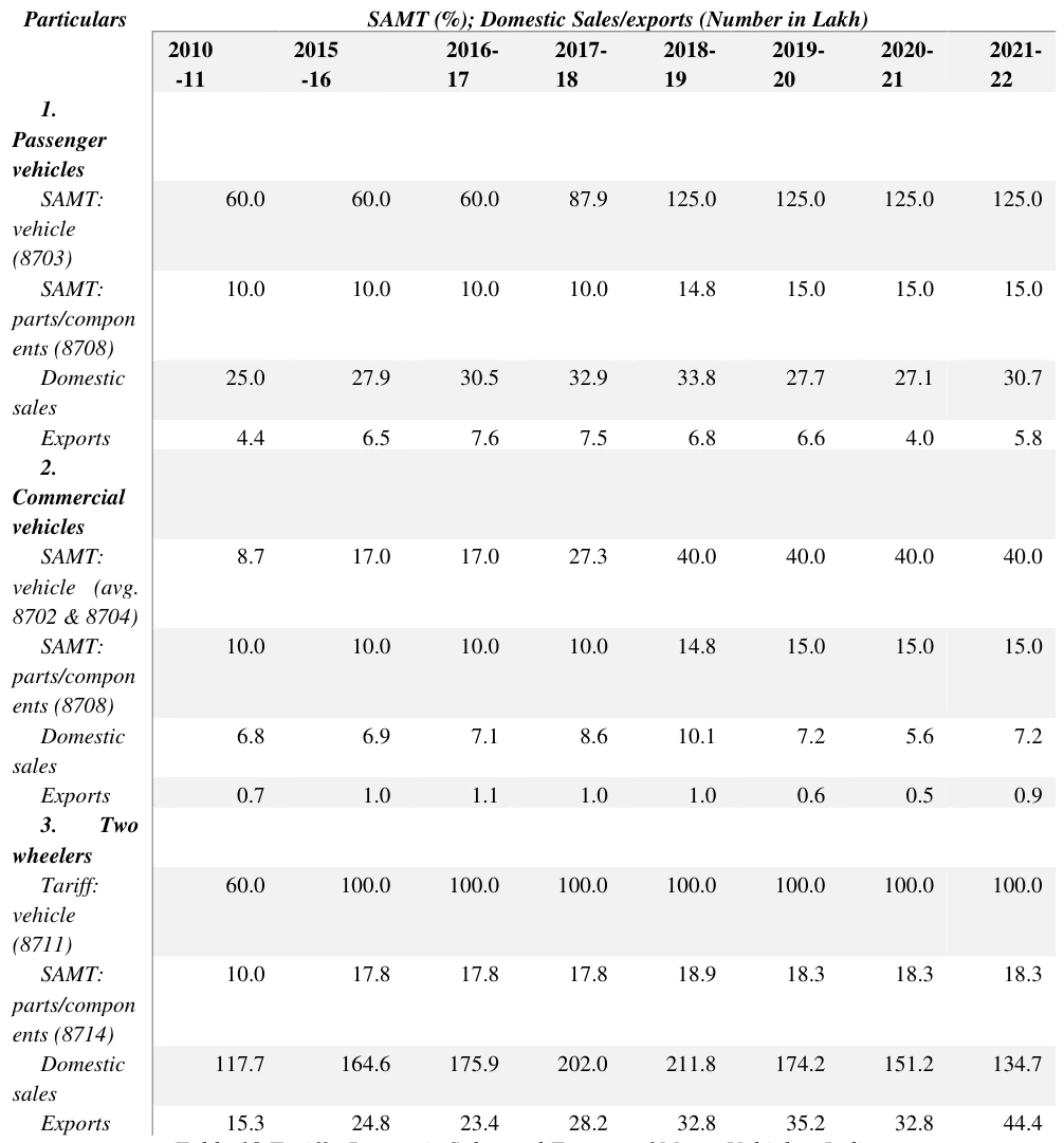
Among the non-agriculture-based manufactures, transport equipment had the steepest increase in tariff between 2010 and 2019 (Fig 3). Tariff on ‘vehicles other than railway or tramway rollingstock, and parts and accessories thereof’ (HS 87) surged to 41.2% in 2019-20 from 19.6% in 2010-11 with tariff on passenger vehicles doubling to 125%. The increase in tariff on commercial vehicles (from 8.5% in 2010-11 to 40% in 2019-20) was even sharper. In both vehicle segments, most of the tariff increase took place during 2017-20 while tariff on two wheelers remained unchanged at 100%. Tariff on parts/components of passenger/commercial vehicles rose from 10% in 2017-18 to 15% 2019-20, while the changes for two wheelers were smaller. Domestic sales in all the three vehicle segments grew till 2018-19. Sales declined in 2019-20 due to poor customer sentiments, liquidity crisis, higher costs due to new safety and environment regulations, etc. (Society of Indian Automobile Manufacturers, Annual Report, 2019-20). Exports of passenger/commercial vehicles declined from 2017-18, while exports of two wheelers grew.
Passenger/commercial vehicles exports though increased in 2021-22 (from the low base), they were lower than the levels attained in the past (Table 18).

Tariffs on vehicles are protective tariffs while tariffs on parts/components increases the cost of production. Both have implications for efficiency. Lower tariffs improve productivity across the value chains in the automotive sector. Trade protection limits firms’ exposure to global best practices. More competitive exposure would force the original equipment manufacturer (OEM) operating in India to bring more customized designs instead of selling last-decade models to Indian consumers. Countries that have closed their markets to Indian vehicle exports in retaliation for high tariffs may be forced to reconsider (Saraf, 2016). The role of FDI and foreign technical collaborations in improving India’s automobile exports is debated. Indian companies have formed collaboration with several foreign OEMs, and they played a vital role as a source of innovation for local auto component supplier firms (Miglani, 2019). The large inflow of FDI in this sector only exploited India’s growing market rather than using India as a base for export-led production (Singh, 2014).
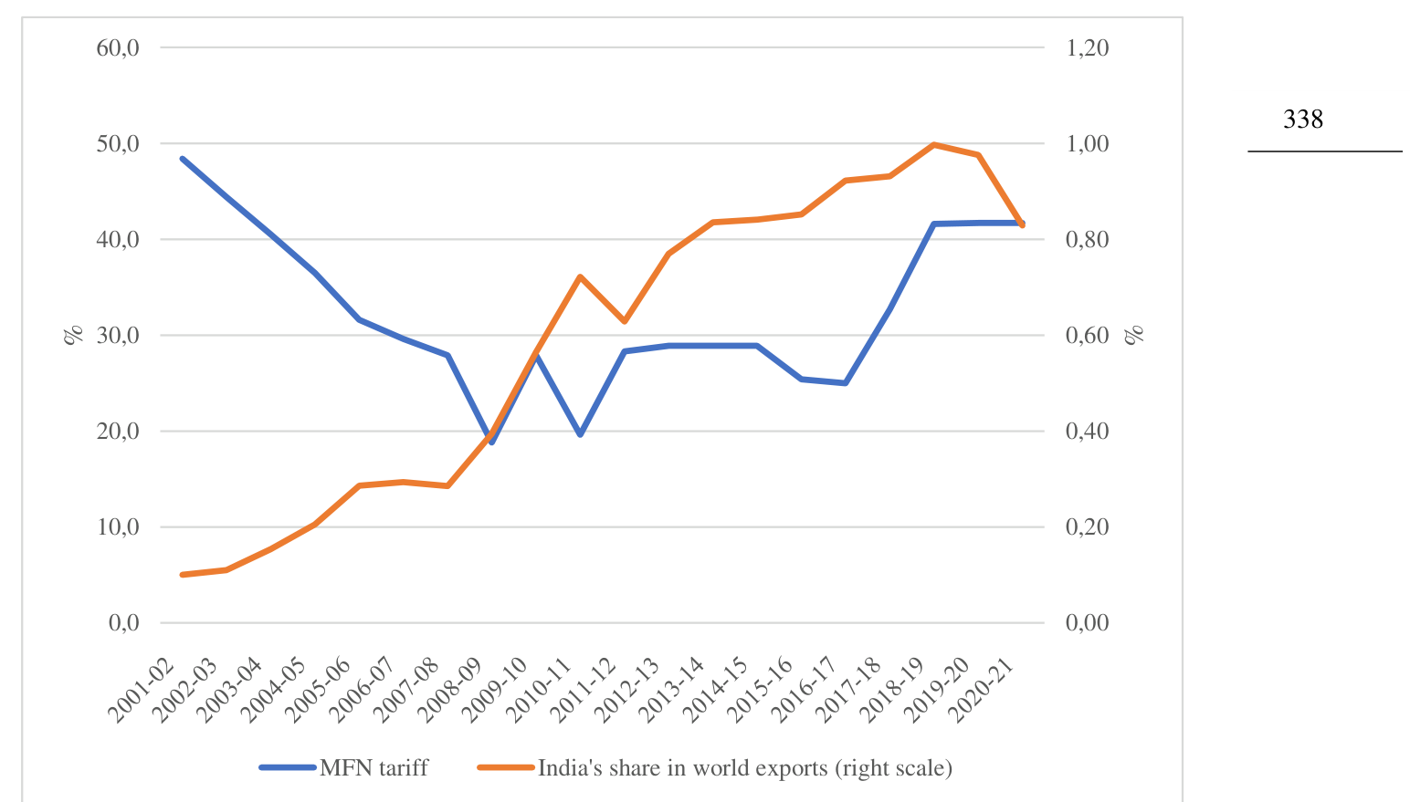
India’s share of world exports improved during 2001-11 with tariff reductions easing input costs and creating competitive conditions in domestic product market. The improvement diminished thereafter with initial flip-flops and later reversal in tariff reforms. The share declined from 2019-20 with the elevated tariffs (Fig 14). The adverse impact of tariff on exports emerges from a gravity model estimation of the determinants of India’s exports of cars using data for 196 partner countries over the 1988-2015 period: the coefficient of nominal applied tariff is negative and statistically significant for compact cars of less than 1000cc (-0.886), while its coefficient in the case of compact cars of greater than 1000cc is insignificant (Athukorala and Veeramani, 2019; 93).
In short, PLI seems to have aided the recent exports of mobile phones, but the low value addition raises a question about the sustainability of domestic manufacturing/assembling. In the vehicles segment, the higher tariffs appear to have abetted the weak exports of passenger cars, which is reinforced by the recent decline in India’s share in world exports of automotive products. Given the evidence, the tariff/subsidy support unlikely would enable domestic manufacturing to endure the impact of the de-globalization: efforts towards re-globalization, unilateral and multilateral, might help. Records of independent India reaffirm the ancient maxim Vanijye Basate Lakshmi (the goddess of prosperity dwells in trade and commerce). By deduction, obstructions in the abode of goddess Lakshmi would bring hardship!
5.2.3. Trade orientation, export performance and economic growth: stylized patterns
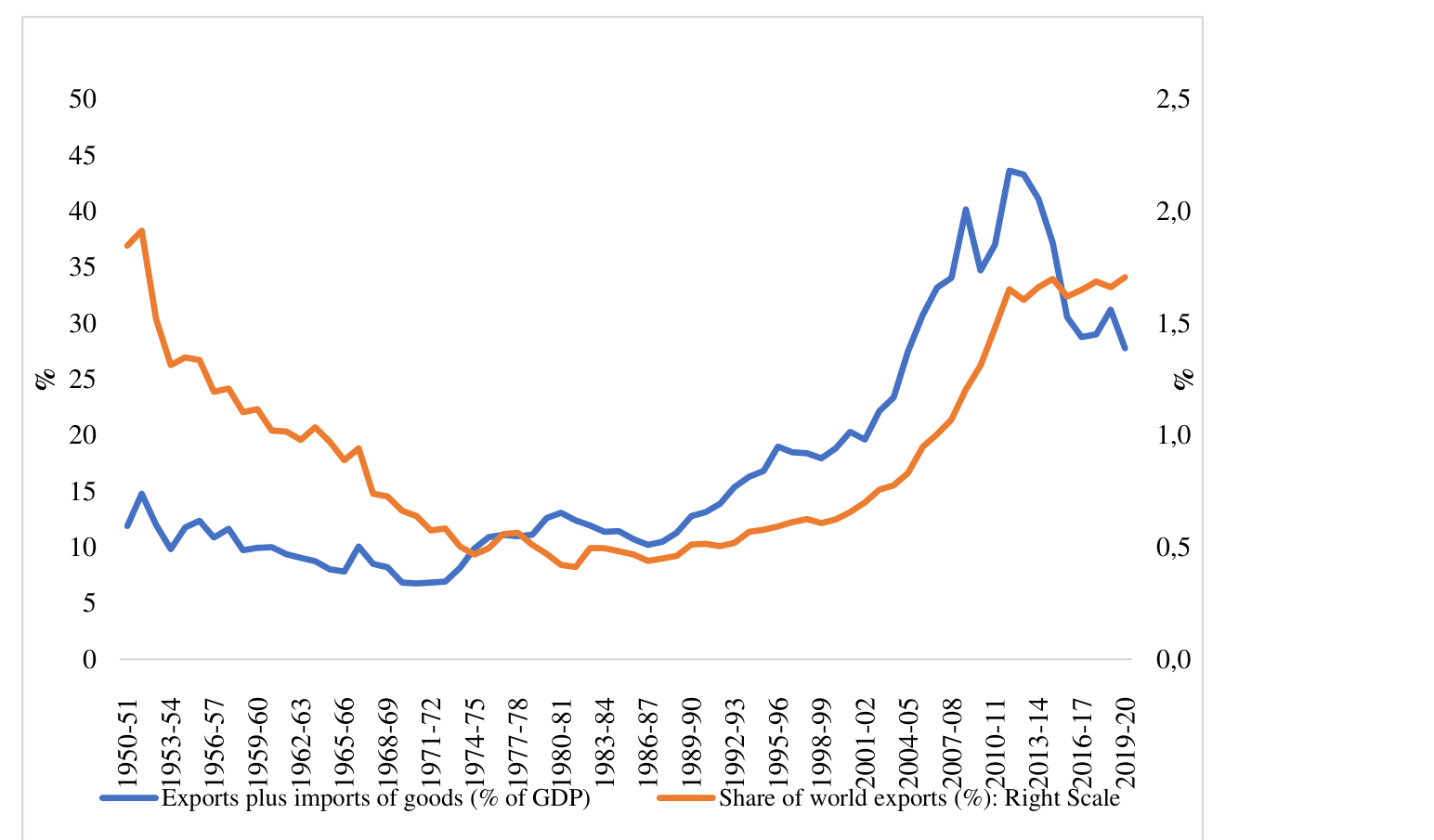
Periods of FTRG, evidenced by policy-induced persistent decline in trade to GDP ratio, had a fall or a virtual stagnation in India’s share of world exports. Export share increased with FTFG, i.e., when the trade-GDP ratio increased (Fig 15). The changes in trade-GDP ratio juxtaposed with the changes in growth rates of GDP over the 1951-2020 period divided into sub-periods according to shifts in trade orientation show that the growth rate accelerated during the FTFG phase (1987-2012) and decelerated during the FTFT phases (1956-1975; and 2012-20).12 When the two FTRG spells are compared, the slide in GDP growth was faster during 2012-20 than in the 1956-75 phase – more pronounced in the PPP series (Table 19). Import curbs, albeit in varying forms, were used in both spells. Erosion in the efforts for human capital formation and innovation were the other growth dampeners of the 2012-20 phase. These are vital for economic growth (Becker, 1962; Schultz, 1975; Galor, 2005; Deming, 2022).
12 The First Plan (1951-56) was largely indifferent to exports and liberal in imports (post-World War-II liberal import policies prevailed). The balance of payment crisis of 1956-57 led to a reversal (Nayyar, 1997; Panagari ya, 2004). The 1975-87 period had huge volatility in GDP growth and the trade-GDP ratio did not show a clear trend.
6. Conclusions
India’s growth suffered jolts during FTRG periods. The loss of competition in domestic product market it entailed and the erosion in other crucial determinants of productivity led the recent decline in the trend growth rate. It also needs a mention that the ‘backseries’ GDP (2011-12 base year), which, among other things, had evoked serious concerns including by 108 economists and social scientists across the world (Azad et al, 2019), also altered the records relevant in the assessment of the growth prospects. The average growth of real GDP for the period from 2005-06 to 2011-12 that was 8.2% in the 2004-05 series changed to 6.9% in the back series. Had the 2004-05 series data for that period been part of the record and had the growth during 2012-20 period not suffered due to FTRG, the GDP growth of 8.6% (for full-fledged OECD membership) perhaps would not have seemed unrealistic. Now it’s fait accompli. Nevertheless, this perspective is important in the discussions on future possibilities. Crucial policy-related factors (tariffs, non-tariff measures, R&D spending, and education) have been covered in this paper. Noninclusion of other factors (notably, public goods other than education) due to the paucity of data is a limitation. With this caveat, some thoughts on what it would take for the goal to make India a developed country by 2047 are given below.
Whether the required GDP growth is 8.6% or 7.4%, most of it should emanate from productivity going by the experience of major economies (Easterly and Levine 2001; Higgins, 2020; Sasaki et al, 2021). Resources must be directed towards boosting the productivity growth in Indian economy: the idea of ‘subsidising the productivity gap’ may not be of much help.
Education, innovation and competition are crucial. Urgent is the need to deploy adequate number of teachers in primary and secondary schools. The 35:1 ratio reportedly used by states for estimating vacancies in government schools (UNESCO, 2021) is too permissive. The PTR norms in the Right to Education Act are aimed at providing for free and compulsory education to children of age 6-14 years: they will not provide for a globally competitive workforce. There are other problems relating to composition, demographic profile, salary structure and workload of teachers, the pedagogy, and teachers training, etc. (UNESCO, 2021). Artificial intelligence (AI) is being seen as a possible solution (UNESCO, 2022). While AI would support the efforts, the improvement that is needed in the educational system to make India a developed country by 2047 would require deployment of teachers as well as financial resources in keeping with the global standards.
R&D intensity is awfully low in agriculture, mining, leather, textiles, food products, and petroleum products, where the activity seems to be thriving under the tariff walls (Fig 11). Governments’ R&D, where they are the sole or main spenders, would need a big leap. Private sector would hopefully increase its R&D, matching business’ in other major economies, if policies require it to ‘make in India in a competitive market’, not a sheltered market.
The key to improving competition in domestic product market lies in easing the import curbs. They might benefit certain interest groups, there are adverse consequences elsewhere.
Exports are important for improving the performance of manufacturing. Factors influencing the efficiency of exporting firms need attention: the routine argument that the slowdown in India’s exports was due to slowdown in global economy is not tenable. The de-globalization may be a cause; it would require efforts for its reversal.
The evidence on the impact of import restrictions on home country economic activity captured from Indian data is relevant for other countries as well. The use of tariffs, subsidies or unilateral trade defence measures may not enable domestic manufacturing weather the impact of the de-globalization. Countries (including India) might benefit if efforts are made, unilateral and multilateral, for the change towards re-globalization.
Loughborough University, Discussion Paper Series.
Research Foundation Occasional Paper 295: 2-47.
Reserve Bank of India Occasional Papers (June).
Export-Import Bank of India Occasional Paper No. 150.
APPENDICES


Accessible table text
| — | Variable | — | — | Data source | — |
|---|---|---|---|---|---|
| — | ADPINI | — | — | WTO. | — |
| — | QM, QX | — | WDI. | — | — |
| — | MGDP, XGDP | — | — | WDI. | — |
| — | REDOL | — | RBI (2021). | — | — |
| — | RFDIR | — | — | Computed using data from RBI (2021) and WDI. | — |
| — | RGDP | — | WDI. | — | — |
| — | RGFCE | — | — | WDI. | — |
| RGERD | RGERD | — | UNESCO (UIS); and GoI, Ministry of Science and Technology (Research and Development Statistics, 2000-01 and 2019-20). | — | — |
| — | REXP | — | — | WDI. | — |
| — | RNOM | — | Computed using data from RBI (2021) and WDI. | — | — |
| — | RPM, RPX | — | — | Computed using data from WDI. | — |
| — | RTFP, CTFP | — | Penn World Table (version 10.0). | — | — |
| — | SAMT | — | — | WDI; data for 1994, 1995 and 1998 have been interpolated. | — |
| — | SSEN | — | WDI. | — | — |